Classifying stars based on raw spectra is virtually impossible. Spectra contain intensity values for thousands of data points, making them difficult to analyze. To combat this problem, we applying dimensionality reduction algorithms to spectra to extract a small number of values that can accurately describe the entire spectra. Stars can then be classified based on these values.
The algorithms used to reduce the dimensionality of the data can have a big effect on the classification results, so we compared the classification accuracy of 3 different dimensionality reduction methods.
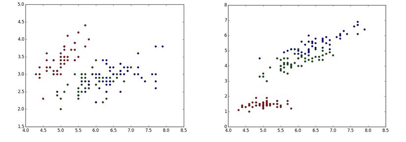
Two different 2D projections of the same 3D data, color-coded by class. Note that in the projection on the right, the classes are separated better than in the projection on the left.
Classification
SDSS and Stellar Spectra
What is SDSS?
The Sloan Digital Sky Survey (or SDSS) is a large-scale sky survey that provides imaging and spectral data for more than three million astronomical objects. The survey covers approximately 1/3 of the sky, which is greater coverage than any previous survey. All data produced by SDSS is publicly available for download. For more information on SDSS, click here.
Our Data
We used stellar spectra selected from SDSS according to the following specifications (following those used in Bu et al.):
K1, K3, K5, K7 stars
Signal-to-noise ratio of at least 10
Full wavelength coverage from 3800 Å to 9000 Å
This resulted in 12,806 total spectra, with 3649 K1 stars, 3532 K3 stars, 3041 K5 stars, and 2584 K5 stars.
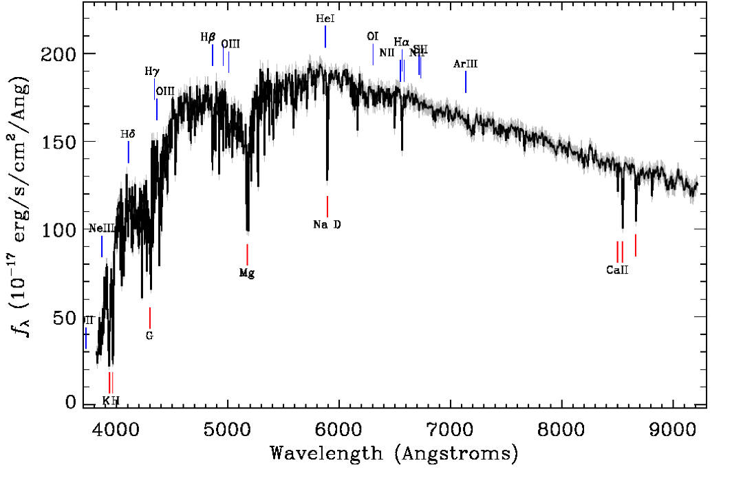
Sample SDSS spectrum of a K1 star. Source: sdss.org.
We then shifted each spectrum to rest-frame wavelengths (to account for redshift) and normalized the total flux. We randomly selected 4 samples of 1500 spectra from the original data, each sample containing 500 K1, 300 K3, 400 K5, and 300 K7 stars. Half of each sample was used as a training set for the classifier, and half was used as a testing set.
Blank
Dimensionality Reduction Algorithms
Dimensionality reduction algorithms embed high-dimensional data into lower dimension surfaces, preserving the inherent structure of the data. We examined three such algorithms in our experiment: Principal Component Analysis (PCA), Isometric Mapping (Isomap), and Locally Linear Embedding (LLE). We implemented PCA, LLE and Isomap using the scikit-learn module in Python. For more information on this module, click here.
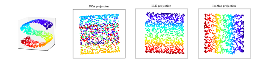
Original data points on a 3D S-shaped manifold projected onto a 2D plane by PCA, LLE and Isomap algorithms. Source: AstroML.org.
Principal Component Analysis
PCA is a linear dimensionality reduction algorithm which projects data onto principal components, or eigenvectors. The principal components that preserve a specified amount of the original variance are selected to make up the lower dimensional space.
Locally Linear Embedding
LLE is a nonlinear embedding algorithm that assumes the original data lies on a locally linear manifold. The algorithm calculates embedding vectors corresponding to this manifold, and then projects the original data onto these embedding vectors.
Isometric Mapping
Isomap is also a nonlinear embedding algorithm. It uses a partially connected graph to calculate local distances between points in a way that preserves the structure locally and globally.
Blank
Embedding
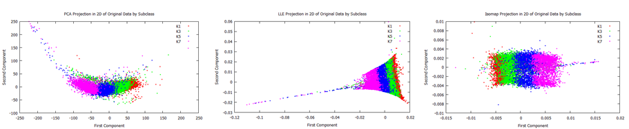
We then projected each of the 4 samples was into 1-10 dimensional space using the PCA, LLE and Isomap algorithms. We examined 2D projections of all of the original data for each algorithm in order to visually examine how well the algorithms separated spectra by subclass. We found that each algorithm noticeably separated subclasses, but there is still significant overlap between each of the subclasses.
Original data points projected onto 2D space by PCA, LLE and Isomap algorithms. Different colors represent K-type subclasses.
Blank
Classification
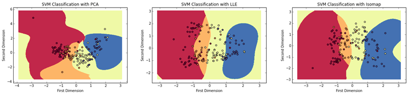
After we reduced the dimensionality of our spectral data, we used a Support Vector Machine (SVM) to classify the spectra. We trained our classifiers on the training data sets and corresponding subclasses, and then predicted the subclasses of spectra in the testing sets.
Contour maps showing SVM classification results for PCA, LLE and Isomap with training points overlaid. Each color in the contour and scatter indicates a subclass: red is K1, orange is K3, yellow is K5 and blue is K7.
Blank
Results
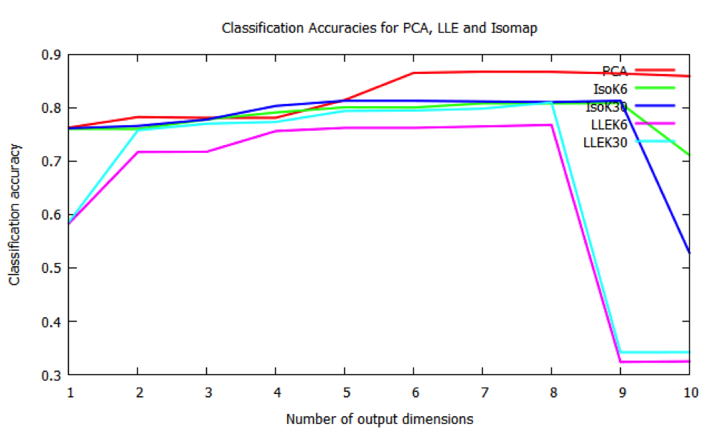
We then determined the accuracy of the classifiers by comparing the assigned subclasses of the testing set to the subclasses given by SDSS. Our results differed significantly to those found in Bu et al. We expected the accuracy of our classifications to peak at around 3 dimensions for Isomap and 4 or 5 dimensions for PCA, and then decrease as the number of output dimensions increases. Additionally, they found Isomap to be more accurate than PCA for all dimensions.
Comparison of accuracies of classifications of PCA, Isomap and LLE projections. Ki indicates i nearest neighbors used in LLE and Isomap algorithms
Our results do not reflect this, which could be for many reasons. We found PCA to be more accurate than Isomap and LLE (which had similar accuracies), and did not decrease as number of output dimensions increased. Even if spectra are overall nonlinear, the distinction between K subclasses could be due to purely linear characteristics, which might explain the high accuracy of PCA. However, this still would not explain why our results are so different from those found by Bu et al., so more investigation is needed.
Blank
Further Work
Our classification results differed from the results obtained by Bu et al. fairly significantly, so we would like to do more work to investigate the accuracy of our results. There are many possible extensions to be done, which could all give more insight into the results we found.
We could perform this same experiment on different types of stars, like M stars for example, or on larger data sets consisting of multiple types of stars, to see how effective our algorithms are in these cases. It would also be interesting to vary the size of our training sets and determine if using smaller testing sets and larger training sets reduces the accuracy of our algorithms.
There are many classification algorithms other than SVM, so experimenting with different classification algorithms would be interesting as well. The LLE and Isomap modules that we used also have training methods that can be used to compute internal parameters before embedding the entire data set. Using these training methods would increase the computational speed, so it would be interesting to see how this might affect our results.
Blank
References
Introduction to astroML: Machine learning for astrophysics, Vanderplas et al, proc. of CIDU, pp. 47-54, 2012. View in ADS
Saul, L. K., & Roweis, S. T. (2001). An introduction
to locally linear embedding. View
Scikit-learn: Machine Learning in Python, Pedregosa et al., JMLR 12, pp. 2825-2830, 2011. View in ADS
Y. D. Bu, F. Q. Chen, and J. C. Pan, "Stellar spectral subclasses classification based on Isomap and SVM," New Astronomy, vol. 28, pp. 35-43, 2014. View in ADS
Zito, T., Wilbert, N., Wiskott, L., Berkes, P. (2009). Modular toolkit for Data Processing (MDP): a Python data processing frame work, Front. Neuroinform. (2008) 2:8. doi:10.3389/neuro.11.008.2008. View
Blank
About Me
I am a math and physics major entering my senior year at Gettysburg College, a liberal arts college in Pennyslvania. I hope to attend graduate school next year in applied mathematics, and I am interested many of the interdisciplinary aspects of math and physics. This summer I participated in an NSF funded REU program through the Center for Interdisciplinary Exploration and Research in Astrophysics (CIERA) at Northwestern University. I am working on an interdisciplinary astronomy project under the supervision of Dr. Ying Wu, a professor in the Electrical Engineering and Computer Science (EECS) department.
Contact: thorte01 {at} gettysburg.edu
This material is based upon work supported by the National Science Foundation under Grant No. AST-1359462, a Research Experiences for Undergraduates (REU) grant awarded to CIERA at Northwestern University. Any opinions, findings, and conclusions or recommendations expressed in this material are those of the author(s) and do not necessarily reflect the views of the National Science Foundation.