
My name is Noah Rivera. I am a physics and computer science double major at California State University San Bernardino.
Over the summer of 2016, I was accepted to participate in the CIERA REU program at Northwestern University in Evanston, IL. During that time, I performed research under the direction of Dr. Michael Schmitt of the physics department at Northwestern.
The majority of my work was learning the astropy python library and how to use the transit method of exoplanet detection to analyze light curves.
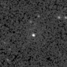
KIC 8462852 is a star in the Cygnus constellation that exhibits an unusually shaped light curve with flux drops of up to 20%. It was imaged as part of NASA's Kepler mission and its anomolous nature was discovered as part of a citizen science project. A follow up report was written with Tabetha Boyajian as its lead author. The star is of spectral type F with radius $1.58 R_{\odot}$ and mass $1.43 M_{\odot}$.
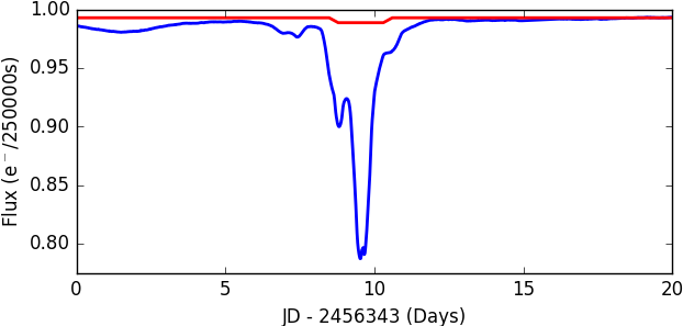
A light curve is a plot of a star's brightness vs time. If an orbiting exoplanet crosses the line of sight between us and its star, some of the star's light will be blocked, producing a dip in its light curve. From this transit, we can determine certain characteristics of the exoplanet.
Assuming a circular orbit and applying Newton's 2nd law and Netwon's Universal Law of Gravitation, an exoplanet's velocity can be found as:$$F_p \; = \; m_p \dot{v_p}^2 \; = \; m_p \frac{v_p^2}{a} \; = \; G \frac{M_* m_p}{a^2}$$ $$\rightarrow v_p \; = \; \sqrt{\frac{G M_*}{a}}$$
The transit time $t$, which corresponds to the length of a dip, can be found by dividing the length of the path a planet travels while crossing the line of sight between us and the planet by $v_p$. This path length can be determined by geometrical analysis. (Figures 3 and 4)
![]()
Assuming an orbit parallel to our line of sight ($b = 0$), $t$ can be found as: $$t = 2 \sqrt{\frac{a^3}{GM_*}} \arcsin{\left( \frac{R_* + R_p}{a} \right) }$$ where $a$ is the semi-major axis (SMA), and $R_*$ and $M_*$ are the radius and mass of the star. $R_p$, which corresponds to the depth of the dip, is proportional to the ratio of projected areas of the star and planet: $$$R_p = R_* \sqrt{\frac{\Delta f}{f}}$$ where $\Delta f / f$ is the proportional change in flux.
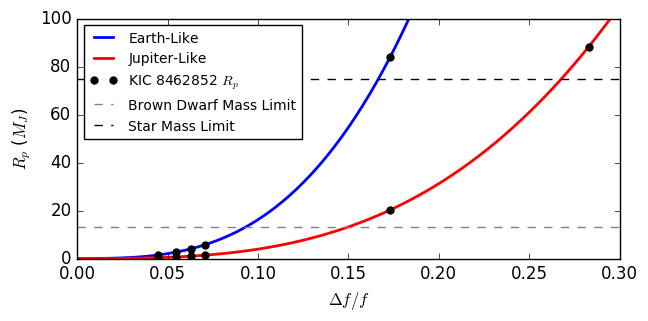
Using depths determined by Boyjian et al, we can calculate potential exoplanet radii. Additionally, by using the density of Earth and Jupiter, we can find the Earth-like and Jupiter-like masses of the potential exoplanets:
| Flux Drop | $R_p$ | $R_p$ | Earth-Like Mass | Earth-Like Mass | Jupiter-Like Mass | Jupiter-Like Mass |
|---|---|---|---|---|---|---|
| % | m | $R_J$ | kg | $M_J$ | kg | $M_J$ |
| 0.2 | 4.92e+07 | 0.70 | 2.75e+27 | 1.45 | 6.62e+26 | 0.35 |
| 0.3 | 6.02e+07 | 0.86 | 5.05e+27 | 2.66 | 1.22e+27 | 0.64 |
| 0.4 | 6.96e+07 | 1.00 | 7.78e+27 | 4.09 | 1.87e+27 | 0.99 |
| 0.5 | 7.78e+07 | 1.11 | 1.09e+28 | 5.72 | 2.62e+27 | 1.38 |
| 3.0 | 1.91e+08 | 2.73 | 1.60e+29 | 84.07 | 3.85e+28 | 20.25 |
| 8.0 | 3.11e+08 | 4.45 | 6.96e+29 | 366.11 | 1.68e+29 | 88.18 |
| 16.0 | 4.40e+08 | 6.29 | 1.97e+30 | 1035.52 | 4.74e+29 | 249.42 |
| 21.0 | 5.04e+08 | 7.21 | 2.96e+30 | 1557.07 | 7.13e+29 | 375.04 |
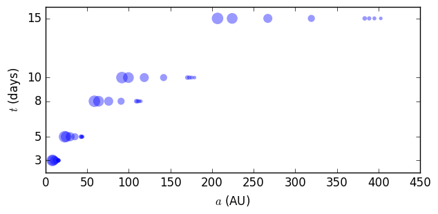
Similarly, we can find the SMA of each exoplanet by solving the first equation for $t$ numerically. Unlike a traditional light curve, KIC 8462852's drops have no clearly defined start or end times so we chose several transit durations (3, 5, 8, 10, and 15 days) for each characteristic depth:
| $R_p$ | $a$ ($t = 3$ days) | $a$ ($t = 5$ days) | $a$ ($t = 8$ days) | $a$ ($t = 10$ days) | $a$ ($t = 15$ days) |
|---|---|---|---|---|---|
| $R_J$ | AU | AU | AU | AU | AU |
| 0.35 | 16.11 | 44.74 | 114.53 | 178.96 | 402.65 |
| 0.64 | 15.80 | 43.89 | 112.36 | 175.56 | 395.01 |
| 0.99 | 15.55 | 43.19 | 110.58 | 172.77 | 388.74 |
| 1.38 | 15.33 | 42.59 | 109.04 | 170.37 | 383.34 |
| 20.25 | 12.77 | 35.48 | 90.82 | 141.91 | 319.29 |
| 88.18 | 10.68 | 29.67 | 75.96 | 118.69 | 267.04 |
| 249.42 | 8.97 | 24.91 | 63.78 | 99.65 | 224.22 |
| 375.04 | 8.27 | 22.96 | 58.78 | 91.85 | 206.66 |
Notice that the $\Delta f / f \geq 3 \%$ would represent planets of Jupiter-like mass larger than the brown dwarf classification limit of $13 M_J$. Additionally, many of the Earth-like mass planets and the larger Jupiter-like mass planets exceed the minimum mass of a star, $0.08 M_\odot = 84 M_J$.
With the calculated masses and SMAs, we set out on comparing them with thoseof actual exoplanets and simulations of exoplanets. Useful data on this information is insufficient, however. Planet formation is not entirely understood and selection effects create bias in observed data.
For example, the transit detection method has an inherent bias due to the probability of visible transit. This probability takes into account the geometric probability that an exoplanet crosses the line of sight between us and its star during a part of its orbit.
By calculating the solid angle subtended by the dashed region in Figure 6 and dividing by the total solid angle, the probability of visible transit is found as: $$P_{transit} \; = \; \frac{\int_0^{2 \pi}{\int_{\pi / 2 - \theta / 2}^{\pi / 2 + \theta / 2}{\sin \phi' \, d\phi' d\theta'}}}{\int_0^{2 \pi}{\int_0^{\pi}{\sin \phi' \, d\phi' d\theta'}}} \; = \; \frac{R_* + R_p}{a}$$ Which clearly depends on mass (which depends on $R_p$) and SMA. From this relation, it is possible for there to be more exoplanets of large SMA or small $R_p$, than we observe. This serves to skew the distributions created from data we record.
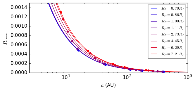
It is worth noting that the probablilities of our calculated exoplanets being visible is extremely small at $P_{transit} ≤ 0.0015$. This is not signifcantly different from the probablity of seeing a planet identical to Earth orbiting a star identical to our Sun at $P_{transit} = 0.005$.
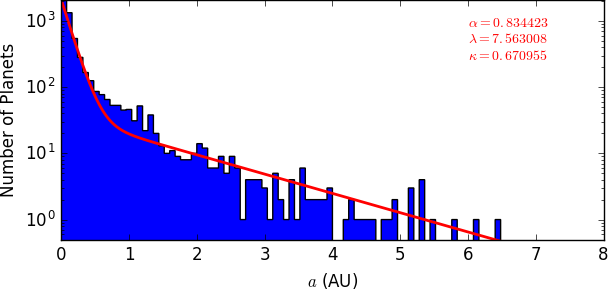
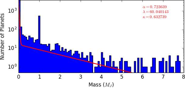
Despite artifacts that can be created by bias, we chose to use observational data of mass and SMA for 5344 exoplanets from The Exoplanet Orbit Database. By examination of the histograms created from this data, the masses and SMAs appear to follow a distribution that is a combination of exponential functions: $$f(x) \; = \; \alpha \lambda e^{-\lambda x} + (1 - \alpha) \kappa e^{-\kappa x}$$
We used the method of maximum likelihood to fit this function to the data. To maximize the likelihood of $f$ given by$$\mathcal{L} (X, \alpha, \lambda, \kappa) \; = \; \prod_{i = 1}^{N} f(x_i, \alpha, \lambda, \kappa)$$ where $X$ is the set of data points, we minimized the -log likelihood:$$-L \; \equiv \; -\log(\mathcal{L} (X, \alpha, \lambda, \kappa)) \; = \; - \sum_{i=1}^N{\log(\alpha \lambda e^{-\lambda x_i} + (1 - \alpha) \kappa e^{-\kappa x_i})}$$by implementing the gradient descent algorithm in Python and finding values for paramters $\alpha, \lambda, \kappa$ such that $-L$ is minimized.
# Implementation of the gradient descent algorithm
def gradientDescent(dfda, x, a, gamma = 1e-1, tolerance = 1e-8):
    # dfda: List of functions representing the partial derivatives of f
    # x:    Parameters of f we are not minimizing with respect to
    # a:    Parameters of f we are minimizing with respect to
    a      = np.array(a)
    a_prev = np.array([float("nan") for i in range(len(a))])

    while(not np.allclose(a, a_prev, rtol = tolerance)):
        a_prev = a
        a      = a - gamma * np.array([dfda[i](x, a) for i in range(len(a))])

return aOur minimization resulted in the parameters $\alpha = 0.83, \lambda = 7.56, \kappa = 0.67$ for the SMA distribution and $\alpha = 0.72, \lambda = 60.0, \kappa = 0.63$ for the mass distribution.
With the fitted functions, we calculated tail probabilities for our calculated SMAs and masses via integration of $f$:$$ P(x) \; = \; \int_{x}^{\infty} f(x')dx' \; = \; \alpha e^{-\lambda x} + (1 - \alpha) e^{-\kappa x}$$
| Mass | Mass Tail Probability | SMA Tail Probability $(t = 3\; days)$ | SMA Tail Probability $(t = 5\; days)$ | SMA Tail Probability $(t = 8\; days)$ | SMA Tail Probability $(t = 10\; days)$ | SMA Tail Probability $(t = 15\; days)$ |
|---|---|---|---|---|---|---|
| $M_J$ | % | % | % | % | % | % |
| 0.35 | 2.22e+01 | 3.36e-04 | 1.52e-12 | 7.00e-33 | 1.18e-51 | 7.76e-117 |
| 0.64 | 1.84e+01 | 4.12e-04 | 2.69e-12 | 3.01e-32 | 1.15e-50 | 1.30e-114 |
| 0.99 | 1.48e+01 | 4.87e-04 | 4.29e-12 | 9.96e-32 | 7.48e-50 | 8.76e-113 |
| 1.38 | 1.16e+01 | 5.64e-04 | 6.42e-12 | 2.79e-31 | 3.75e-49 | 3.28e-111 |
| 20.25 | 7.53e-05 | 3.14e-03 | 7.61e-10 | 5.69e-26 | 7.39e-41 | 1.52e-92 |
| 88.18 | 1.62e-23 | 1.28e-02 | 3.74e-08 | 1.22e-21 | 4.31e-34 | 2.54e-77 |
| 249.42 | 8.00e-68 | 4.03e-02 | 9.11e-07 | 4.31e-18 | 1.52e-28 | 7.64e-65 |
| 375.04 | 2.41e-102 | 6.46e-02 | 3.37e-06 | 1.23e-16 | 2.85e-26 | 9.98e-60 |
With the assumption that exoplanet mass and SMA are independent, we multiplied the tail-probabilities of each (Table 3) to obtain the probablity that each of our planets would be drawn from observed distributions (Table 4).
| Mass | Planet Probability $(t = 3\; days)$ | Planet Probability $(t = 5\; days)$ | Planet Probability $(t = 8\; days)$ | Planet Probability $(t = 10\; days)$ | Planet Probability $(t = 15\; days)$ |
|---|---|---|---|---|---|
| $M_J$ | % | % | % | % | % |
| 0.35 | 7.44e-05 | 3.37e-13 | 1.55e-33 | 2.62e-52 | 1.72e-117 |
| 0.64 | 7.59e-05 | 4.96e-13 | 5.54e-33 | 2.12e-51 | 2.40e-115 |
| 0.99 | 7.22e-05 | 6.36e-13 | 1.47e-32 | 1.11e-50 | 1.30e-113 |
| 1.38 | 6.51e-05 | 7.42e-13 | 3.23e-32 | 4.33e-50 | 3.80e-112 |
| 20.25 | 2.37e-09 | 5.73e-16 | 4.28e-32 | 5.57e-47 | 1.14e-98 |
| 88.18 | 2.07e-27 | 6.06e-33 | 1.97e-46 | 6.99e-59 | 4.11e-102 |
| 249.42 | 3.22e-71 | 7.28e-76 | 3.45e-87 | 1.21e-97 | 6.11e-134 |
| 375.04 | 1.56e-105 | 8.14e-110 | 2.97e-120 | 6.88e-130 | 2.41e-163 |
These probabilities ranged from $2.41 \times 10^{-163}$ (for $M_p = 375 M_J$ and $a = 207$AU) to $7.59 \times 10^{-5}$ (for $M_p = 0.64 M_J$ and $a = 16$ AU) %.
For the larger masses and SMAs corresponding to the largest dips, extremely low probabilities are further proof that the exoplanet theory is unlikely. The probabilities are not as remote for the smaller dips with reasonable masses and SMAs, but their light curve is inconsistent with typical transits.
Future work could involve using these results to calculate how many planets of these extreme values we might observer with future missions and telescopes such as TESS, WFIRST, GMT, and TMT.