How Mathematics Describes Life
The circle of life is something we have all heard of from somewhere, but we don't usually try to calculate it. For some time we have been working on analyzing a predator-prey model to better understand how mathematics can describe life, in particular the interaction between two different species (a predator and a prey). The model we are analyzing is called the Holling-Tanner model, and it can't be solved analytically. The Holling-Tanner model is a very common model in population dynamics because it is a simple descriptor of how predators and prey interact. The model is a system of differential equations that is controlled by constants of how the species interact. This model is a generalized math concept, so it can describe any predator prey interaction given the right constants; from lions and zebras to white blood cells and diseases.The model is a system of two differential equations with solution properties described by three parameters which are characteristics of the interacting species and their environment. The model is not specific to any particular set of species and so can describe predator-prey species ranging from lions and zebras to white blood cells and infections.
One thing all these systems have in common is they all have critical points. A critical point is a value for both populations that keeps both populations constant. It is a pair of equilibrium populations for the predator and the prey; this is important because for such a point the right hand sides for both differential equations are equal to zero. For this model there are two critical points, a predator free critical point and a coexistence critical point. Most of the analysis we did is on the coexistence critical point because the predator free critical point is always unstable and frankly less interesting than the coexistence critical point.
What we did is consider two regimes for the differential equations, large $B$ and small $B$. $B$, $A$, and $C$ are constants in the differential equations that control the nature of the solution where $B$ measures the responsiveness of the predators population to change; as $B$ gets larger the predators become more responsive. $A$ represents predation of the prey, and $C$ represents the satiation point of the prey population. For the large $B$ case we were able to approximate the system of differential equations by a single scalar equation. For the small $B$ case we were able to predict the limit cycle, as well as look at the type of solution all regimes of $B$ give us. The limit cycle is what I referred to earlier as the circle of life; it is a process of the predator and prey populations growing and shrinking periodically. This model has a limit cycle in the regime of small $B$, that we solved for numerically. With some assumptions to reduce the differential equations, we were able to create a system of equations and unknowns to predict the behavior of the limit cycle for small
Why
One fundamental problem in population dynamics is the predator-prey
problem. In its simplest form there are only two species - the prey
and the predator. The predators survive by devouring the prey. When
the prey population is large, the predators will increase because
there is more for them to eat. Conversely, when the prey population is
small the predator population will decrease because they do not have
enough to eat. In many instances the decrease of the predator population
causes the prey to recover and then subsequently the predator population
will increase again. The result is a cyclic behavior of the predators
and the prey with the predators lagging the prey. While this problem
has been stated in terms of population dynamics, similar behavior
can occur at the cellular level, for example white blood cells acting
as predators and some external intrusion, i.e., an infection, acting
as the prey.
Let $P(t)$ and $V(t)$ represent the populations of the prey and predators,
respectively, as functions of time $t$. Many different predator-prey
models have been proposed and studied, but one very important model
is called the Holling-Tanner model. In its most general form this model
is a coupled system of two differential equations,
$$
\frac{dP}{dt}=P(\alpha-\beta P-A\frac{V}{P+C}) \,, \quad \frac{dV}{dt}=BV(1-\gamma \frac{V}{P}) \, ,
$$
where $\alpha$, $\beta$, $\gamma$, $A$, $B$ and $C$ are
positive constants. This model can be simplified by appropriate
nondimensionalization of $P$, $V$ and $t$ resulting in a set of equations
where $\alpha$, $\beta$ and $\gamma$ are set to 1,
$$
\frac{dP}{dt}=P(1- P-A\frac{V}{P+C}) \,, \quad \frac{dV}{dt}=Bv(1- \frac{V}{P}) \, .
$$
In order to understand what these equations mean, consider first the $P$
equation.
The term in parenthesis is the net birth rate per unit population.
For small values of $P$ and $V$ this term is just one and is just the
natural birth rate of the species. The next term $-P$ represents
a crowding effect. For any species, if the population is too large
then intraspecies competition for a scarce resource decreases
the birth rate (hence the negative sign). The last term is predation
(again with a minus sign) and represents the decrease in the prey
population when they interact with predators. The denominator
in this term represents a satiation effect and simply says that
there are limits to how much the predators can consume, i.e., for large
$P$ predation (per unit population) decreases.
Next consider the $V$ equation. Again, the term in parenthesis
is the net birth rate per unit population for the predators and
the equation simply states that when the predator population is greater
than the prey population $V>P$ there is not enough prey for the predators
to consume and their population decreases (term in parenthesis is negative), whereas if $V< P$ the predator population will grow (term in parenthesis is positive). This system is a highly nonlinear system of differential equations and in general there is no analytic solution - it can only be solved numerically. However, it can be analyzed mathematically by looking for critical (equilibrium) populations where the right hand side of each equation is zero. If you find such a point then the populations are in equilibrium, since their time derivative is zero.
Note that the only solutions of interest are when $P(V)\ge 0 )$ since $P$ and $V$ represent populations. Negative values of $P$ or $V$ describe non-physical solutions. It is easy to see that one such critical point is $(P,V)=(1,0)$. This is called the predator-free state since $V=0$. Simple math analysis shows that the predator-free state is always unstable, small perturbations will lead to a solution which moves away from the predator-free state ($V$ grows). A second critical point $(P_{*},V_{*})$ with $V_{*}=P_{*}>0$
also exists. The right
hand side of the second equation is zero when $V=P$ so that we must
have $V_{*}=P_{*}$. We can then solve for $P_{*}$ from a simple
algebraic manipulation of the right hand side of the $P$ equation.
This critical point is called the coexistence critical point
since the two species exist together in equilibrium. For a large
range of parameter values the coexistence critical point is
unstable, and the solution will evolve to a periodic solution
$P(t),V(t)$ representing cyclic growth and decline of the
two species. This solution is called a limit cycle because
it is the limit (as $t\rightarrow \infty$) of general initial conditions
and because it is periodic (cyclic).
The limit cycle can be studied in two ways, (i) compute and plot
$P(t)$ and $V(t)$ and (ii) consider the curve in the $P-V$ plane
which this periodic solution traces out (by eliminating $t$).
This last approach is called a phase plane analysis and is useful
because you can directly see the relationship between $P$ and $V$.
In general, the limit cycle and solutions in general can only be
attained through numerical computation. However, in this project
I show how you can mathematically analyze the system in the two
regimes (i) $B$ small and (ii) $B$ large. In the first case I show
how you can get a simple analytic approximation to the limit cycle.
In the second case I show how you can reduce the system of equations
from two equations to just one scalar
How
To look at the stability of the critical points of these linear, autonomous differential equations we used two methods. The first is to solve for the direction field numerically. The second is to make a Jacobian matrix and find the eigenvalues. The equation that describes them is the following: $$ \frac{dP}{dt} = P\left(1-P-\frac{AV}{P+C}\right) $$ $$ \frac{dV}{dt} = BV(1-\frac{V}{P}) $$ These two equation describe the growth rate of the two populations with respect to time and each other. When these two equations equal zero is when they are in equilibrium (have constant population); that is what the critical point describes. There are two critical points, when $(V,P) = (0,1)$ and $(V,P) = (P_c,P_c)$. The $P_c$ we are looking at is positive and real; the value describes what population the two species can coexist. To calculate the critical point we can do the following. $$\frac{dP}{dt} = P\left(1-P-\frac{AV}{P+C}\right) = 0~~~~~~~ \frac{P(1-P)(P+C)-AP^2}{P+C} = 0$$ We set $V = P$ because that is where the critical point is, and now we can simply solve for the numerator using the quadratic formula; $\gamma = A + C$. $$P_c = \frac{1-\gamma}{2} + \frac{\sqrt{(1-\gamma)^2 + 4C}}{2}$$ To confirm what kind of critical points we found we checked the Jacobian matrix of the differential equations and then found their eigenvalues. Depending on the eigenvalues we can determine the type of critical point. The Jacobian matrix of two differential equations can be described as the following: $$\frac{dP}{dt} = P\left(1-P-\frac{AV}{P+C}\right) = f$$ $$\frac{dV}{dt} = BV(1-\frac{V}{P}) = g$$ $$J = \begin{bmatrix} \frac{\partial f}{\partial P} & \frac{\partial f}{\partial V}\\ \frac{\partial g}{\partial P} & \frac{\partial g}{\partial V} \end{bmatrix} $$ We can then use this information to categorize the solutions for all regimes of all the constants. To approximate these differential equations into a single scalar equation we started with the rate of change of the predators. $$ \frac{dV}{dt} = BV(1-\frac{V}{P}) $$ If we assume that $B$ is large then we can bring it to the other side of the equation, and we can assume at large enough $B$: $$ \frac{1}{B} \frac{dV}{dt}=V(1-\frac{V}{P})\approx 0 $$ Since we are not investigating the predator free state we can remove that as a solution. $$(1-\frac{V}{P})\approx 0$$ What is left is the assumtion $V\approx P$ and we can then have a single scalar equation that describes the rate of change of the two populations. $$\frac{dP}{dt} = P\left(1-P-\frac{AP}{P+C}\right) $$
To understand how we predicted the shape of the limit cycle for small $B$, the first step is to reformulate the system so that the small number $B$ is in front of one of the derivatives. To do this make the change of variables $\tau=Bt $, so that we now get the system of equations $$ B\frac{dP}{d \tau}=P(1-P-A\frac{V}{P+C})\, , \quad \frac{dV}{d \tau}=V(1-\frac{V}{P}) \, . $$ Now consider the direction field for this system.
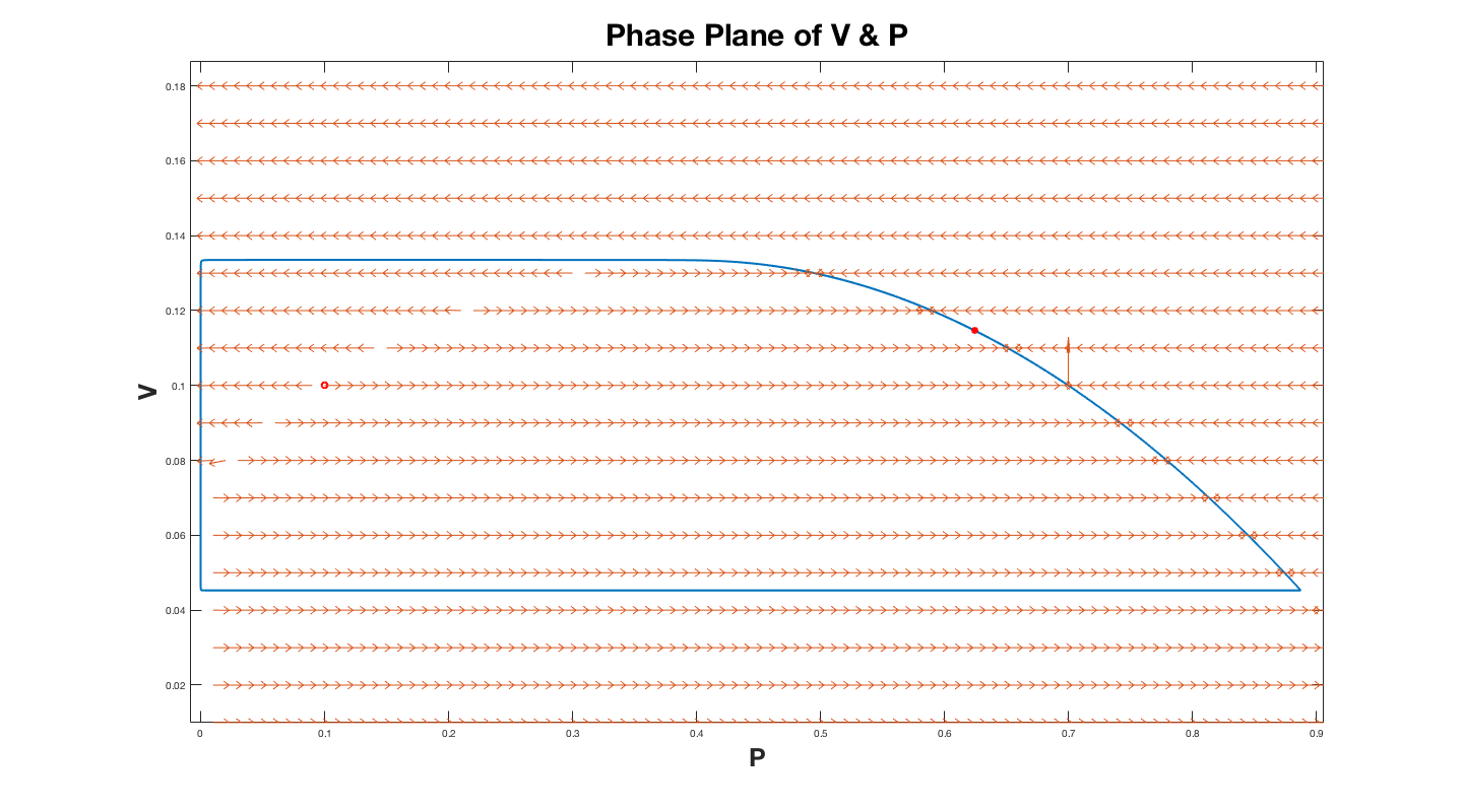 The plot above is for $B = 10^{-5}$. In the plot above the halo red dot represents the critical point, and the solid red dot represents where the numerical solution stopped solving for the limit cycle.
Since for $P$ we now
have $B$ in the denominator
$(\dfrac{dP}{d \tau}=\dfrac{P}{B}(1-P-A\dfrac{V}{P+C})\, )$,
we expect the direction field to be nearly horizontal ($dP$ predominates)
unless either $P$ or $(1-P-A\dfrac{V}{P+C})$ is close to zero.
The equation $1-P-A\dfrac{V}{P+C}=0$ describes a
downward facing parabola. Thus, portions of
the limit cycle where $V$ really changes (not horizontal in the $P-V$ plane)
have to be either near this parabola or have $P$ small.
Consider first the parabola. Along the right branch of the parabola
$dV$ is positive so that the limit cycle will include a curve very
close (not exact of course) to the right branch of the parabola.
When the maximum of the parabola is reached (call it $V_{max}$) the
limit cycle can no longer follow the parabola since the
parabola turns down
but the direction field still points upward ($dV$ still positive).
The only possibility is that the limit cycle is now nearly horizontal until
it reaches a small value of $P$ ($P_{turn}$)
when it will turn down. We approximate
this turning point by looking at a point where the direction field
points in the $45^{\circ}$ direction and $V=V_{max}$
($dP=dV$ and $V=V_{max}$ - one equation and one unknown for $P_{turn}$).
Next consider how $V$ changes when $P$ is small.
Since $dP$ will now be small, we expect this part
of the limit cycle to be nearly vertical ($dV$ predominates).
For small $P$ we can
get an approximate equation for $\dfrac{dP}{dV}$ which we can solve.
$$
\frac{dP}{dV} = -\frac{P(1-\frac{A}{C}V)}{B\frac{V^2}{P}}
$$
To solve we will seperate the variables and integrate and set $\frac{dP}{dV} = -1$. This will give us two equations for $P$ as a function of $V$ which will allow us to solve for $V_{small}$. This will also allow us to find $P_{turn 2}$. The limit cycle
will follow this nearly vertical line until it turns back again at
$P_{turn2}$, and $V_{small}$. When it turns again it will be nearly
horizontal until it intersects the parabola
at $P=P_{intersect}$. We can then calculate $P_{intersect}$ by setting the equation for the parabola equal to $V_{min}$. These steps allow us to construct a good approximation to the
limit cycle for small
Results
To showcase the results we will display many plots. The first of which is a region plot that characterizes the solutions to the Holling-Tanner model.
.png)
.png)
It is well known that a critical point can be classified
into several different possibilities. These possibilities
are called nodes, spirals and saddles. Nodes and
spirals can also be either stable or unstable.
Limit cycles occur when the coexistence critical point
is an unstable spiral. Since there are three parameters
(A, B, and C) in order to visualize regions where
the critical point has different behavior we reduced the
visualization to two dimensions. We did this by freezing
the value of the critical point (for the figures above the
critical point was (0.1,0.1)). The value of the critical
point does not depend on B, only on A. For the
left most figure we considered different values
of A and B, computing what C would have to be in order
to keep the critical point fixed. For the right most figure
we did the same but giving C and computing A.
If this resulted in negative parameters we did not try
to classify the critical point, rather we just considered
the case unphysical. The region of the unstable spiral
is where cyclic behavior occurs and there is where limit cycles occur.
In the plot below$ P(t)$ is the population of prey, $V(t)$ is the population
of predators and in blue we plot $P$ obtained from the
single scalar equation that I derived for the large $B$ case.
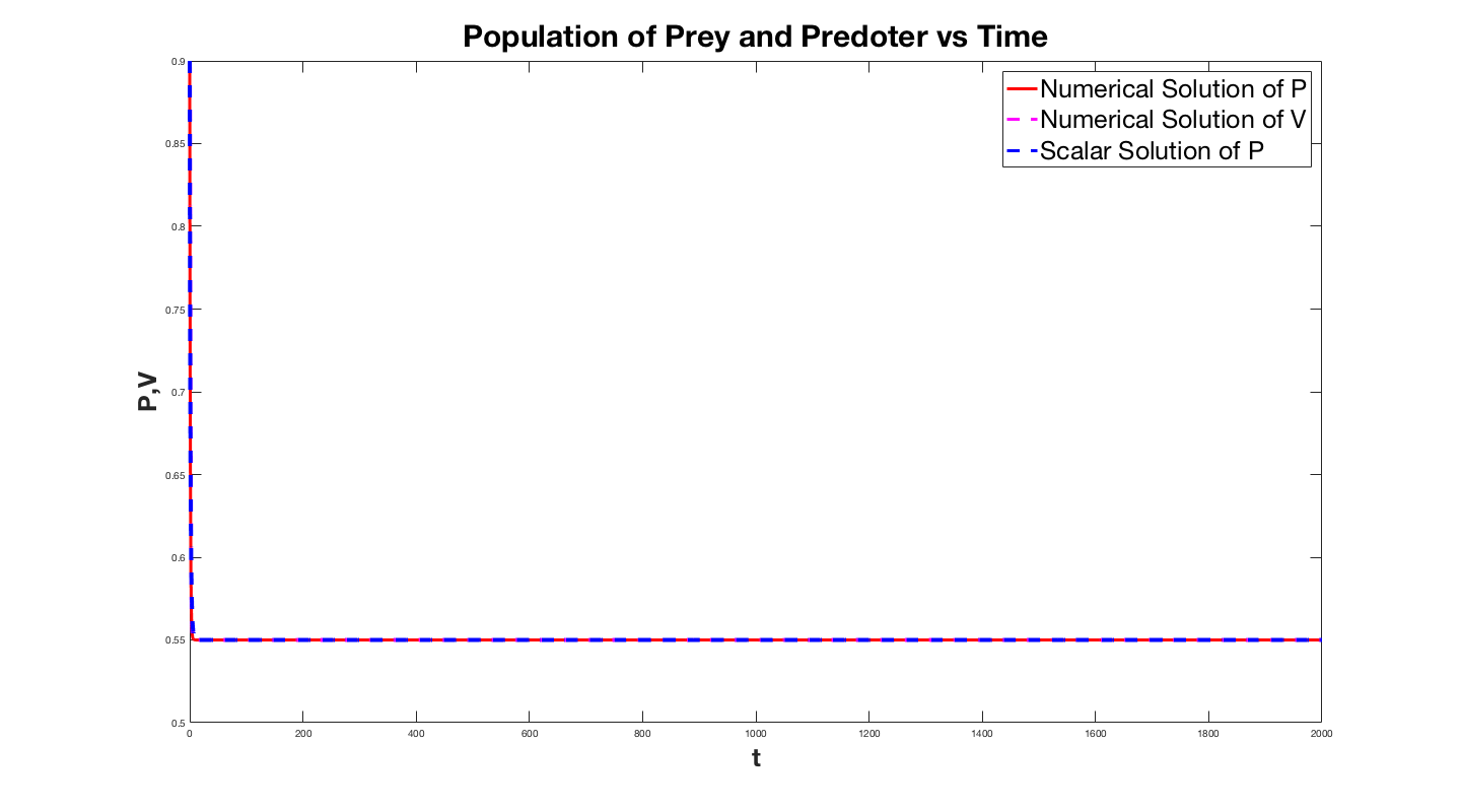
The first plot is for B=2 and the solution for the system almost
immediately latches on to the solution to the single
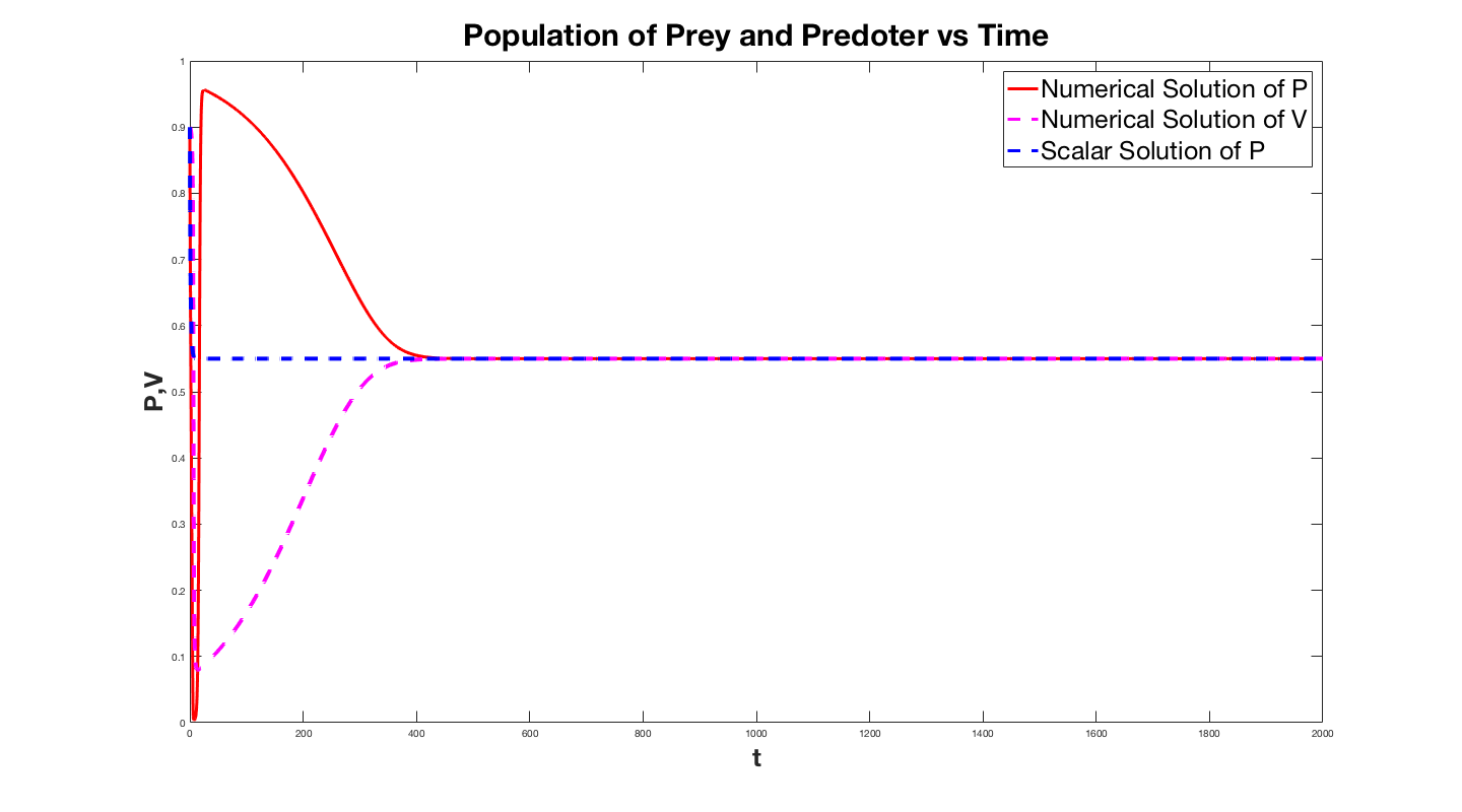
equation. The second plot is for small B and while
asymptotically the solution to the system approaches that
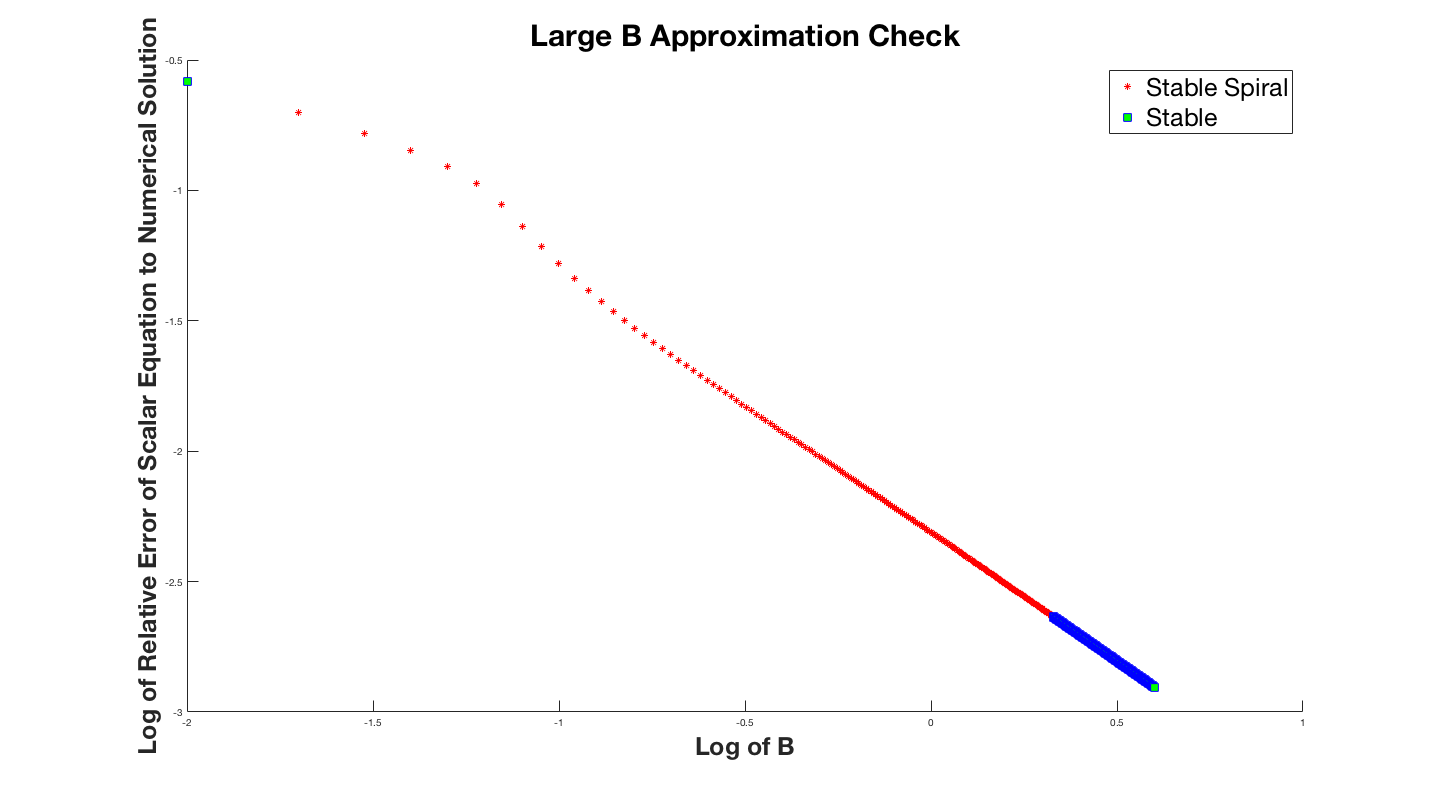
of the scalar equation. The lower plot is the same curve except for $B=0.001$. This displays how the solution degradates as $B$ gets smaller. We infact took an interest in how much the solution degredates as a function $B$, so we plotted the relative error of the solutions as a function of $B$.
For the small $B$ regime we were able to analytically predict the limit cycle without solving the system of differential equations. The plot below shows the two solutions overlayed on top of eachother.
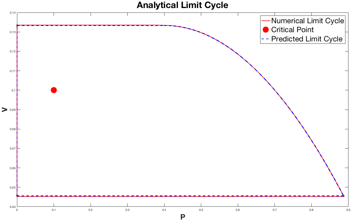
The plot above shows the two solutions in the $V-P$ plane to better illistrate the limit cycle. This result is very exiciting because it gives us an analytical method to approximate the limit cycle. The plot above has the critical point $(0.1,0.1)$, and $B = 10^{-5}$. Notice that the approximation is not perfect; at the top and bottom horizontal regions the approximation is slightly off of the numerical solution. The more we raise the value of $B$ the larger these errors become.
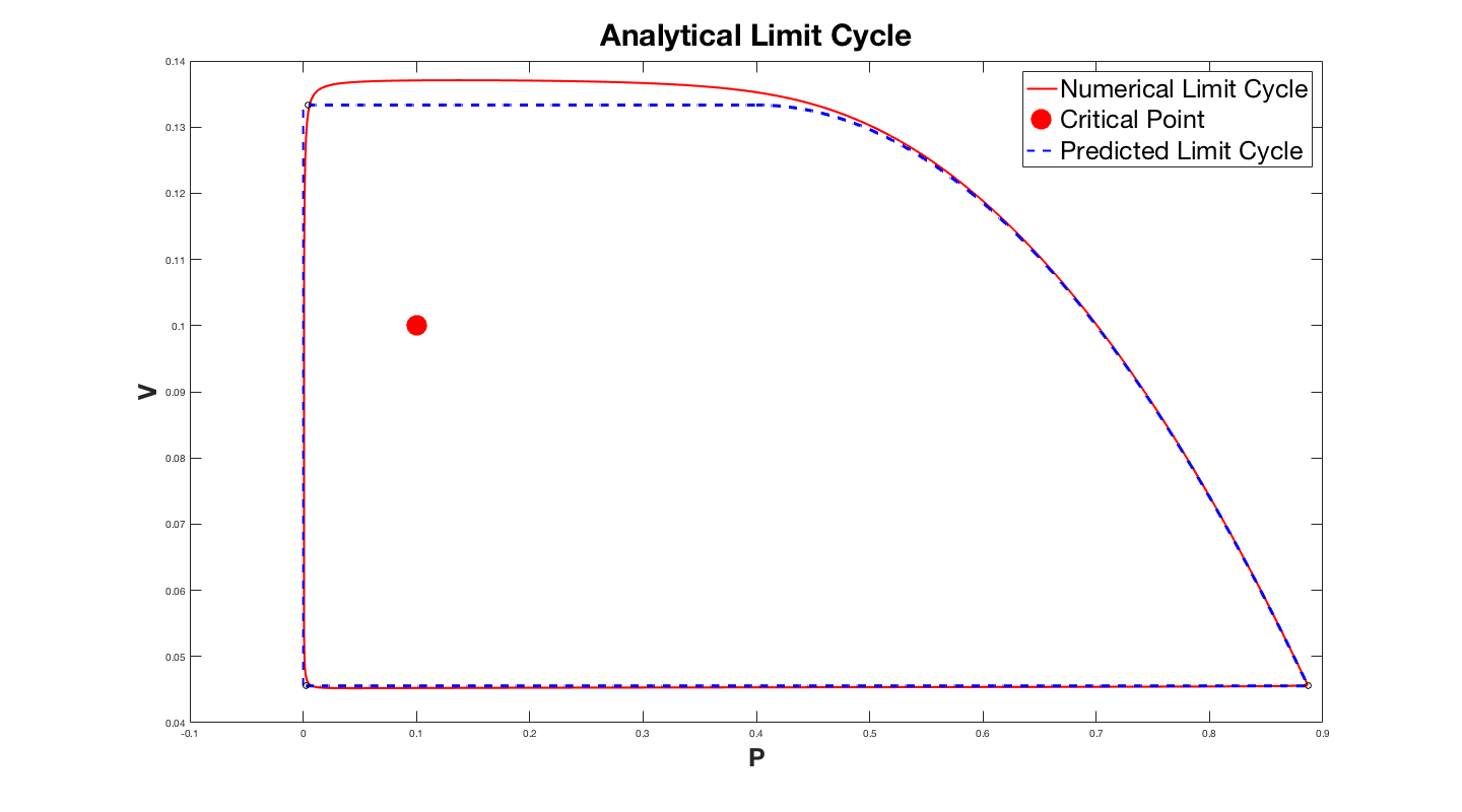
The plot above has the parameter $B = 10^{-3}$. The error might become larger, but is still a reasonable approximation. This method can be used to better understand the system of equations, and the limit cycle. Hopefully this might even inspire new ideas for other models.
Acknowledgements
This approach was suggested by Applied Mathematics Professors Vladimir A. Volpert and Alvin Bayliss. I also want to acknowledge help from Applied Math graduate student Eric A. Autry.