Building and Characterizing a Comprehensive Library of High-z Star Formation Histories
Owen Gonzales
Claude-André Faucher-Giguère, Guochao Sun, Andrew Marszewski
Understanding the evolution of high-redshift galaxies is crucial to developing our knowledge of the early universe. With the launch of the James Webb Space Telescope (JWST), we have been able to peer deeper into space and earlier into time than ever before. This has led to multiple lines of evidence that suggest that low-mass, high-z galaxies possess highly variable, or "bursty" star formation histories (SFHs) (Sun et al. 2023, Muñoz et al. 2023).
Bursty SFHs are also predicted by multiple modern cosmological zoom-in simulations, such as the Feedback in Realistic Environments (FIRE) project (Faucher-Giguère 2018). Simulations like FIRE are able to simultaneously resolve a galaxy's interstellar medium (ISM) as well as its large scale cosmological environment. This allows for explicit modeling of a wide variety of physical processes which influence that galaxy's SFH. Stellar winds, radiation pressure, core collapse and type Ia supernovae, and even supermassive black hole (SMBH) feedback can all be captured by the FIRE simulations (Hopkins et al. 2014).
Star formation histories can provide insight into observable properties of the galaxies which produce them (Dressler et al. 2023). Thus, by building a connection between simulated SFHs and the observable properties of real galaxies, we can better understand how low-mass, high-z galaxies evolve and interact with each other and their environment. With this project we begin building this connection by creating a comprehensive, publicly available, and user-friendly library of simulated SFHs and other relevant properties. Data for this library come from the High Redshift suite of the FIRE-2 simulations. We use the data contained in the library to characterize the burstiness of the obtained SFHs, as well as to compare them against theoretical models.
We consider three final redshifts from the high-z suite: z=5.024, z=7.000, and z=9.000. We use the gizmo_analysis package (Wetzel and Garrison-Kimmel 2020) to read in the data from the final snapshots of 25 zoom-in simulations. For this library, we adopt the ``archaeological approach'' to compute the SFH: Using a theoretical galactic outer edge of 0.2Rvir (virial radius), we identify the star particles belonging to each galaxy, as well as when those particles formed. A fraction of 0.2 is assumed to capture only star particles belonging to the galaxy itself, rather than those belonging to satellite galaxies/subhalos. The archaeological approach is not sensitive to galactic mergers or other forms of accretion and assumes that all star particles that are present in the galaxy, at the last snapshot, have always been part of that galaxy. Although the FIRE-2 simulations do possess pointers to allow tracking of star particles between snapshots (Wetzel et al. 2023), for our purposes, these approximations are sufficient.
Once identified, the particles are placed into time bins of width Δt, each weighted by the mass of each star particle. The resulting sum gives the mass formed within each time bin in units of M⊙. Dividing this mass by the size of the bin yields the SFH in units of M_*/M⊙/yr. In this library, we provide three bin sizes: Δt1 = 1 Myr, Δt2 = 5 Myr, Δt3 = 10 Myr. We record other useful properties such as the galactic coordinates (x, y, z) in physical kpc, number of particles Nparticles, virial mass Mvir, mass as a function of time M*(t), and specific star formation rate sSFR(t) = SFR(t)/M*(t). Our calculation of M*(t) takes into account mass loss as the stars age and can be written as
$M_*(t) = \sum_N m_N(t)A(t - t_{\mathrm{ form, N}})$
where $A(t)$ is the observed fractional stellar mass loss function of the FIRE-2 simulations, $m_N$ is the mass of the $N$th star particle in the galaxy, and $t_{\mathrm{form, N}}$ is the time at which that star particle formed. The resulting library contains over 1200 galaxies across 25 independent simulations.
Once written to files, we adopt methods from Tacchella et al (2022) to quantify the level of "burstiness" in each SFH. This method involves fitting a second order polynomial in logarithmic space to the SFH. Since we choose a continuous function as our model, we must remove SFHs with many points of discontinuity (i.e. many points of zero SFR). This is done by applying an somewhat arbitrary mass cut of $M_* \geq 10^7M_\odot$, chosen to remove most of the zero-SFH galaxies while removing none of the highly continuous ones.
We next subtract the fitted polynomial from the data to obtain residuals $\delta (t)$. These residuals are binned into a histogram, and a Gaussian fit over the resulting distribution. We perform KS-test for normality on the observed $\delta (t)$ distribution, against the Gaussian fit obtained, to compute a p-value. Galaxies whose Gaussian fits produce p-values of $p\leq 0.4$ are rejected. This threshold produced the best results after visual inspection of the resulting distributions. For the remaining well-fit galaxies, the standard deviation of this Gaussian $\sigma_\delta$ can be thought of us as a measure of the average deviation from equilibrium, or the strength of the average "burst". More detail on this method can be found in Tacchella et al (2022). An example of this method is shown below in Figure 1.
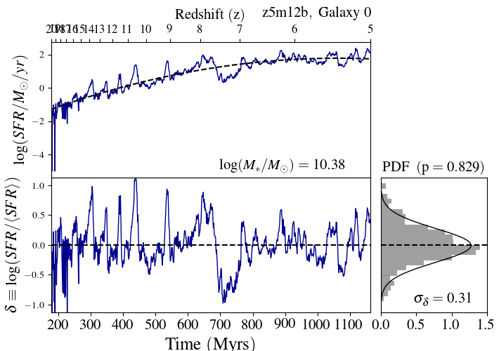
Figure 1: σδ characterization of burstiness for the host galaxy of simulation z5m12b. The standard deviation of the residuals serves as a quantitative measure of "burstiness".
In order to obtain information about the fluctuation timescales, we computed the power spectral densities (PSDs) of each SFH. The PSD gives a measure of how much power, relative to the full signal, is included in each component frequency of the true signal. This can give insight into the physical processes driving the signal. This was done using the welch function from the scipy package. We then fit a power law model to each PSD. The power law index $\alpha$ determines the steepness of the model. In this context, this corresponds to the relative importance of long-timescale vs. short-timescale fluctuations. Similarly, the amplitude $A$ determines the total amount of power in the signal, with higher numbers representing stronger fluctuations overall. Comparison of these two parameters give us insight into how the shape and amplitude of the SFH are influenced by stellar mass.
We also aim to quantitatively determine how well various non-parametric models of SFHs fit our data. We borrow non-parametric model definitions from Tacchella et al (2022), who provide non-parametric models for both bursty and continuous SFHs. These models define six bins, evenly spaced in logarithmic time from $z=20$ to $z=10$ with the first bin set at a fixed size of 10Myrs to capture recent star forming activities. The ratio of the SFR of any bin to the bin before it is draw from a Student's t-distribution (Eq. 2) with the parameter $\nu$ fixed at $2.0$.
$T(x; \nu, \sigma) = \frac{\Gamma(\frac{\nu+1}{2})}{\Gamma(\frac{\nu}{2})\sqrt{\pi\nu\sigma^2}}\left(1+\frac{x^2}{\nu\sigma^2}\right)^{-\frac{\nu+1}{2}}$
We define three different SFH prior distributions based on the parameter $\sigma$: ``flexible'' priors ($\sigma = 1.0$), ``moderate'' priors ($\sigma = 0.3$), and ``restrictive'' priors ($\sigma = 0.1$). We note that our flexible priors are identical to the ``bursty'' priors from Tacchella et al (2022), and our moderate priors are identical to their ``continuous'' priors.
Following their example, we consider the data from $z=20$ to $z=10$, separated into identical time bins. We determine the ratios between adjacent bins by calculating the ratios between the averages within these bins. Lastly, we attempt to compute a rough probability that a given SFH was drawn from each of the two distributions using the following equation:
$P = \prod_{n=1}^5\int_{\Delta_n-0.01}^{\Delta_n+0.01}T(\Delta)d\Delta$
Here $P$ is the combined probability of randomly drawing all of the observed ratios $\Delta_n$ given a probability distribution of $T(\Delta)$. The probability of each individual ratio is determined using the integral expression. The $\pm 0.01$ is included in the bounds only as a way to avoid infinitesimals when computing probabilities and is arbitrarily chosen to be a number well below sensitivity of the models. Lastly, the product of each of the probabilities of the five ratios represents the full probability of the SFH. We compute $P_f$, $P_m$, and $P_r$, the probabilities given flexible, moderate, and restrictive priors, respectively.
We find that σδ is highly dependent on the stellar mass of the galaxy, with σδ more than halving over 3 dex of stellar mass, as shown in Figure 2. This is likely due to the deeper gravitational potential wells of the larger galaxies. A deeper gravitational potential well makes it more difficult for mechanisms like stellar feedback and minor mergers to have a disruptive effect on the galaxy, thus their imprint on the variability of these SFHs is softened. In the regime of galactic masses considererd, our data are well fit by a linear model in log-log space with slope α = -0.18 ± 0.02
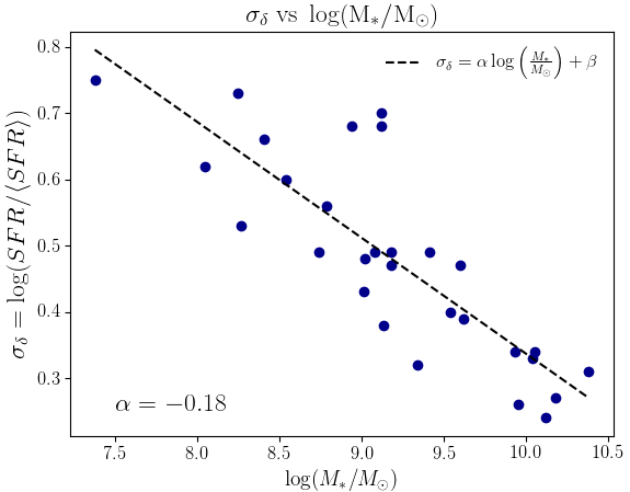
Figure 2: σδ vs M* relationship. Galaxies appear to get less bursty as mass increases.
Interestingly, these results differ from those found by Pallottini and Ferrara. (2023), who claim a roughly constant value of σδ = 0.24, independent of galactic mass. Not only do they find an absence of a relationship between these two properties, but their values of σδ are systematically lower than the ones found in this work, being as low as σδ = 0.19. This is in contrast to our analysis, which finds values as low as σδ = 0.24 [log(M*/M⊙) = 10.12] and as high as σδ [log(M*/M⊙) = 7.38]. Similarly to their work, we do however find that our PDFs are symmetric, which could indicate that periods of intense star formation are followed by periods of relative quiescence, potentially pointing to a type of self-regulating process (Pallottini and Ferrara. 2023). Because galaxies with many points of zero SFR artificially skew the distribution towards zero, the data points in Figure 3 are only a fraction of the total number. Characterization of the burstiness of the poorly fit galaxies will require alternative methods.
These results are further supported by analysis of the PSDs and their power law fits. Like above, we find an inverse relationship between α and log(M*/M⊙). Galaxy mass appears to determine the lower limit of α with this parameter reaching a minimum of -0.4 when log(M*/M⊙) ≅ 7.0, yet only reaching a minimum of -1.6 when log(M*/M⊙) ≅ 10.3. This indicates that, on average, low-mass galaxies experience relatively more intense fluctuations on shorter time scales while high-mass galaxies are more tranquil. Similarly, the amplitudes of high-mass and low-mass galaxies differ by over 1 dex, indicating that low-mass galaxies experience more intense burstiness in general. These results can be seen below in Figure 3
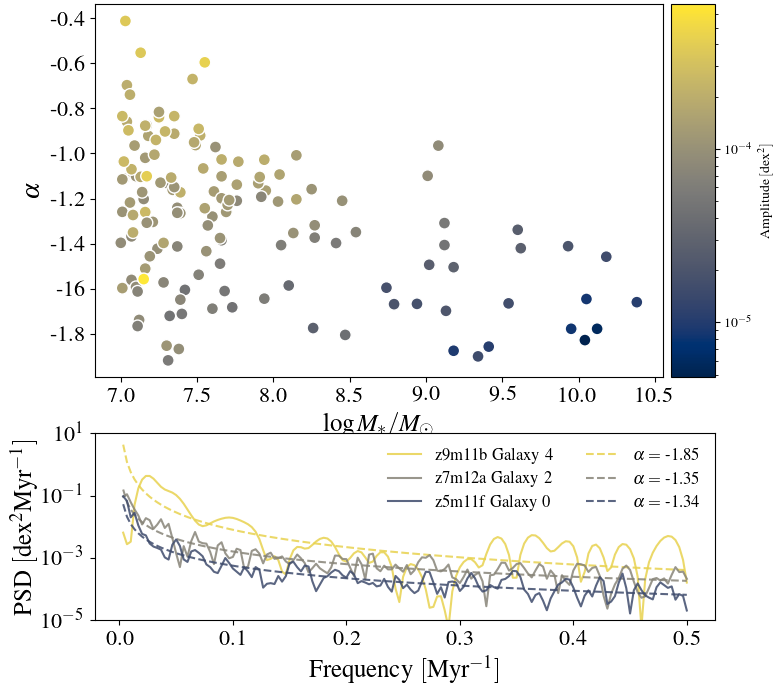
Figure 3: α vs log(M*/M⊙) relationship, along with PSDs and power law fits. Maximum steepness increases with mass. High-mass galaxies experience relatively weaker bursts dominated by low frequency oscillations.
Additionally, we find that 86.2% of galaxies for which this analysis was preformed are best fit by a model SFH with moderate priors. The sample of SFHs generated in Tacchella et al (2022) using their "bursty" model exhibit more extreme fluctuations, with the SFRs of adjacent bins having ratios of up to three orders of magnitude, while our data produce ratios just over 1.0 in extreme cases (Figure 4). This is a surprising result, given the undoubtedly bursty nature of the FIRE-2 SFHs. This may indicate that parametric SFH models may require less flexibility than previously assumed to adequately capture the behavior of real galaxies. Alternatively, six bins may be insufficient to capture the behavior of these galaxies, smoothing out much of the variability, and almost entirely removing the short timescale fluctuations. Further analysis of this discrepancy will require more work to be done on this topic.
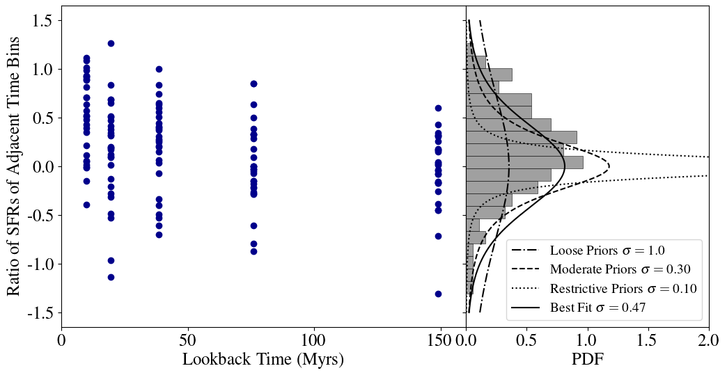
Figure 4: Ratios between adjacent SFH bins and t-distribution fits. Each blue dot is located along the x-axis at the boundary between the two bins of which it is an average. Its y-axis position is the ratio between bins. Results are represented in a histogram. The σ parameter represents the optimal level of flexibility required to reproduce the results seen in the FIRE-2 high-z simulations.
In future work we aim to make this library publicly available and crate a python package to read in the data and perform function on it. Additionally, we will look at mass inflows and outflows from the galaxies in order to connect SFHs to their larger cosmological evnironment. Lastly, we will extract spectral energy distributions (SEDs) from each galaxy. Finding correlations between SFH behavior and SED may allow us to disentangle the histories of real high-z galaxies observed by JWST by comparing their SEDs to ones which are produced by a known classification of SFH. This has the potential to greatly increase our knowledge of high-z galaxies, and thus our understanding of how the early universe behaved, and why it look the way it does today.
Hi! I'm Owen Gonzales and I am a rising senior at Wesleyan University double
majoring in physics and astronomy. My work this past summer focused on developing theoretical understanding of galactic
star formation histories using data from the FIRE project. I also have done research in radio astronomy, using CO line
emission to dynamically measure the host stars of gas-bearing debris disks. Apart from astronomy, I am an avid weightlifter,
runner and musician.
I would like to thank Claude-André Faucher-Giguère, Guochao (Jason) Sun, and
Andy Marszewski for their support and guidance on this project. I would also like to thank Aaron Geller, Emily Leiner,
and the Northwestern CIERA REU program for the opportunity to conduct this research. This has been an incredible summer
and I am very grateful to have been able to research at CIERA with amazing people.
This material is based upon work supported by the National Science Foundation under grant No. AST 2149425, a Research Experiences for Undergraduates (REU) grant awarded to CIERA at Northwestern University. Any opinions, findings, and conclusions or recommendations expressed in this material are those of the author(s) and do not necessarily reflect the views of the National Science Foundation.