Predicting observation quality

The quality of any observation is quantified by the five-sigma depth for point sources at a particular time and place (m₅). This value corresponds to the brightness of the dimmest source that could be detected. M₅ is given by the following formula:

Here, C_m is a constant based on telescope properties, t_vis is the observation time (usually 30 seconds for LSST), and k_m is the atmospheric extinction coefficient, a constant based on the filter being used (values found in section 3.1.2 of Ivezic et al. 2018). This leaves only seeing (θ_eff) and sky brightness (m_sky) to be predicted.

Determining seeing and sky brightness

Seeing is affected by a number of factors that increase scattering of light in the atmosphere. The most important is airmass, or how much atmosphere the light is traveling through. Airmass depends upon the angle of elevation of an observation. Other factors affecting seeing include temperature, humidity, turbulence, etc.

Sky brightness is a measure of ambient light measured everywhere in the viewing window. This light comes from the sun, the moon, stars, and radiation from the atmosphere itself. Sky brightness also depends on the filter being used.

A tool to predict observing conditions

LSST’s Operations Simulator (OpSim) provides θ_eff and m_sky for each observation in a simulated ten-year run. It does not provide any information on locations and times outside of these limited observations. Generalizing OpSim’s code, our tool provides θ_eff, m_sky and m₅ anywhere, anytime.

Kilonova example and implications for future work

As an example of the insight one could gain with this tool, we plotted the five-sigma depth on an arbitrary night at an arbitrary time over the 90% confidence area for a simulated kilonova event. The colored region is the localization area. The top row is a binary neutron star merger detected with two GW detectors. The middle row is a neutron star - black hole merger with four detectors online, and the bottom row is a different neutron star - black hole merger with three detectors. Viewing conditions in the Y-filter are shown at three different times on the morning of January 1st, 2030.

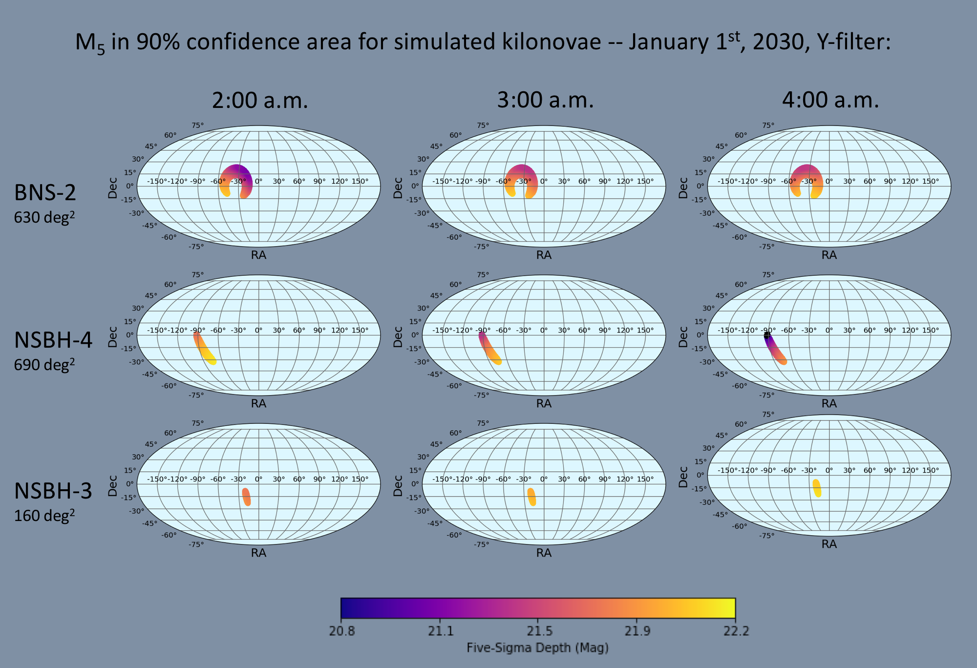
Analysis of these results reveals important implications for follow-up strategies. If BNS-2 were detected at 2:00 a.m., this figure suggests that viewing should begin in the southwest corner of localization and perhaps jump to the southeast corner before tiling the northern segment. If NSBH-4 were detected at 2:00 a.m., LSST should perhaps begin viewing at the northern end because conditions there will deteriorate more rapidly than in the southern end. If NSBH-3 were detected at 2:00 a.m., the small localization area suggests that one could wait until viewing conditions improved at around 4:00 a.m. before beginning observation at all.

In general, the tool reveals that the conditions for observing a particular event may be significantly anisotropic and variable in time within the necessary viewing area, confirming that effective tiling strategies should consider viewing conditions when determining where to look and when.