The Effects of Neutrino Decay on Oscillation Probabilities
Kayla Leonard, Dr. André de Gouvêa
.
| Abstract | About the Neutrino | Neutrino Decay | Contact |
Since there are three types of neutrinos that a particle can start and end as, there are 9 transition probabilities to calculate.

We calculated these probabilities under the assumption that decay is allowed. The probabilities are functions of many variables:
- Δ : mass differences ( Δij = ai - aj )
- b : "lifetimes" of mass sates
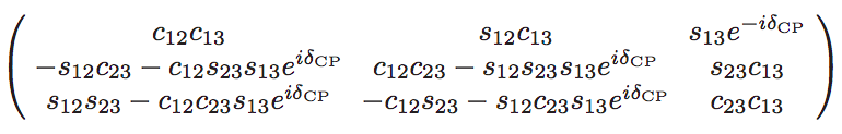
- θ : mixing angles
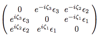
- ε, ζ : decay parameters
The Hamiltonian
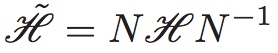
when

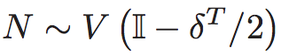
Several of the parameters have been measured by experimental data. For example, we think we know the mixing angles within a few degrees. Unless otherwise noted, we used
There are many free variables; however, some combinations don't make physical sense. There are 3 things that can happen to the total number of particles in the beam:
(1) constant: conservation of probability; Hamiltonian matrix is Hermitian
(2) increase: no physics currently could explain this
(3) decrease: some particles decay; Hamilotonian matrix is non-Hermitian
This third case is the one we are interested in.
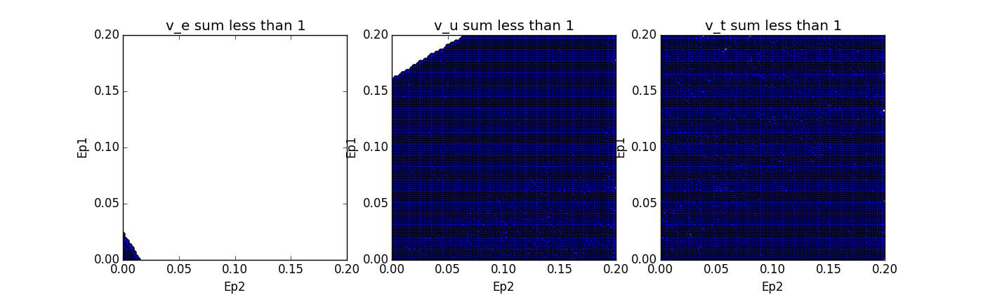
We tested many combinations of the unknown parameters to see what constraints we could determine. In the sample plots below, the blue dots indicate allowed epsilon regions. These epsilon values will not make the number of particles exceed 1. You can see that the different parameters listed below affect the allowed epsilon values.
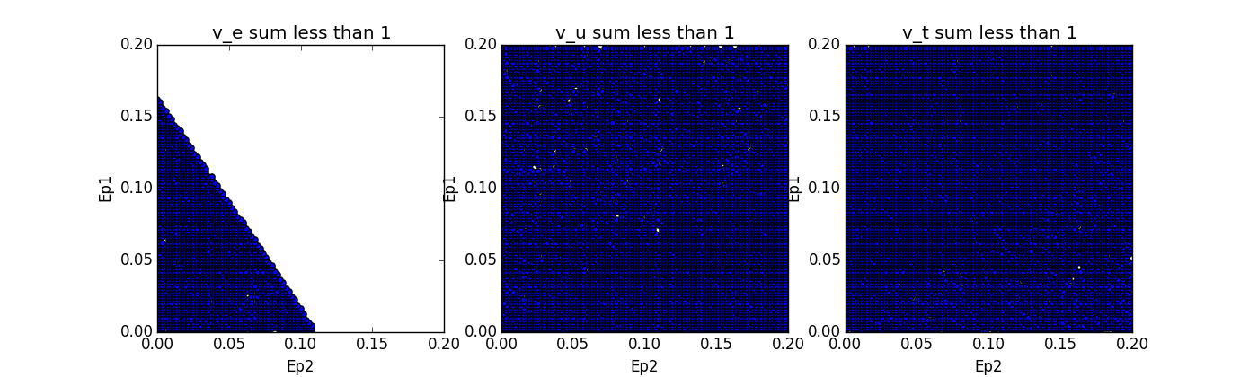
a1=1, a2=2, a3=31,
b1=0, b2=0, b3=3,
ζ1=π/3, ζ2=π/3, ζ3=π/3
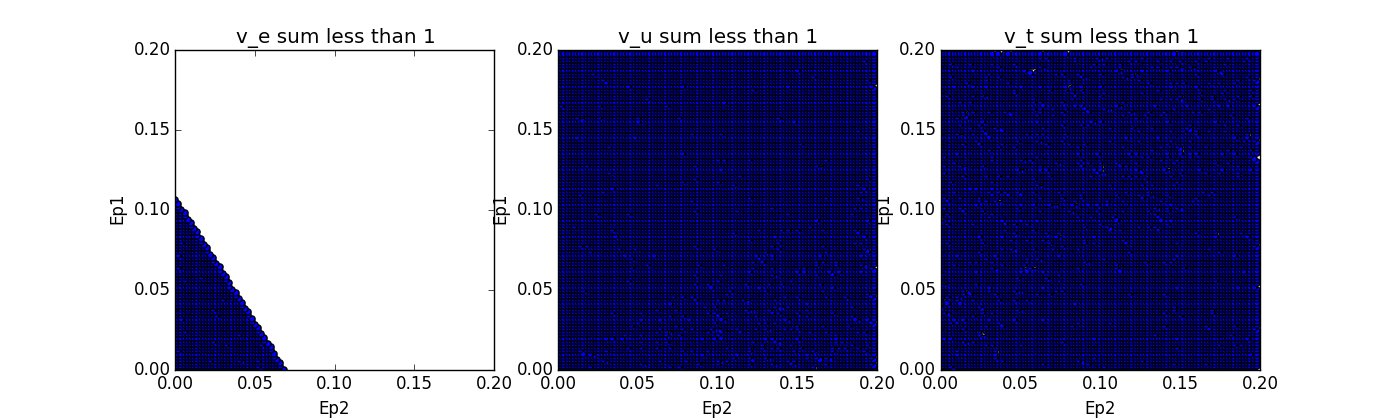
a1=1, a2=2, a3=31,
b1=0, b2=0, b3=3,
ζ1=π, ζ2=π, ζ3=π
a1=1, a2=2, a3=31,
b1=0, b2=0, b3=100,
ζ1=π, ζ2=π, ζ3=π/3
After determining the maximum epsilon values that are allowed in step 3, we examined the impact it could have on the oscillation probabilities. In the sample plot below, the region between the lines represents the possible oscillation possibilities. The green line indicates no decay, and the blue line indicates maximum decay.
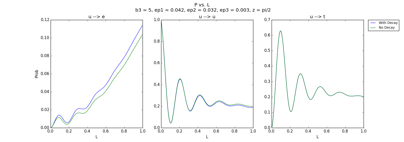
a1=1, a2=2, a3=31, b1=0, b2=0, b3=5, ζ1=π/2, ζ2=π/2, ζ3=π/2, ε1=.042, ε2=.032, ε3=.003
The existence of neutrino decay being proven or disproven would be hindered by an inability to isolate its effects from the effects of other parameters.
We look at the effects as a function of energy, because this is something that can vary from experiment to experiment. Different experiments have sensitivity to different energy ranges, so combining data from solar experiments and long baseline experiments (NOvA, DUNE, etc.) will help construct a more complete picture over a range of energies.
In the plots below, the blue line represents a probability with no additional effects. The red line indicates the effects of maximum decay; it changes the position of the line. When we change b values (the green line) the amplitude changes, so this would not be confused with decay. The effects of changing Δ12/Δ13 may be difficult to distinguish from decay in P(u → e) and P(u → u). However, in the P(u → t) channel, these two effects shift the probabilities in opposite directions, and thus should be distinguishable.
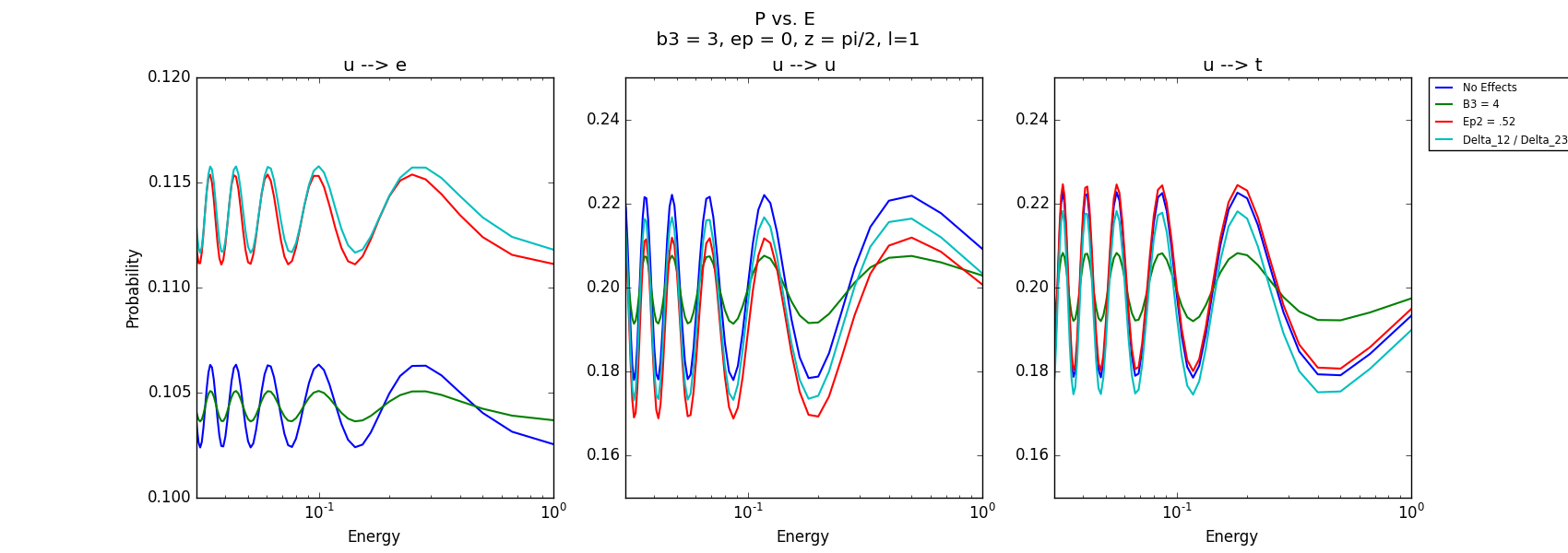
a1=1, a2=2, a3=31, b1=0, b2=0, b3=3, ζ1=π/2, ζ2=π/2, ζ3=π/2, ε1=0, ε2=0, ε3=0
* these values are used unless listed diferently in the legend on the right of the image
With 14 free parameters, there are far too many dimensions to explore all possible oscillation probabilities now. However, we can determine that some combinations should allow for the effects of neutrino decay to be measurable depending on :
- if decay exists, and if so, what the decay parameters are
- the sensitivity of future experiments
- other measurements, such as mass differences
To test for CP Invariance, we compare the oscillation probabilities of a certain transition with the probability of their anti-particles' transition. For example, P( e → u ) minus P( e → u ). You can see in the plot below that when we do this, we see that the resulting differences are non-zero. This means that if neutrino decay were proven true, it would be a new source of CP violation. This would be an important clue in understanding the why the universe has more matter than antimatter. Sources of CP violation are required in explanations of matter-antimatter asymmetry, therefore neutrino decay may be a contributing factor in the lepton sector.
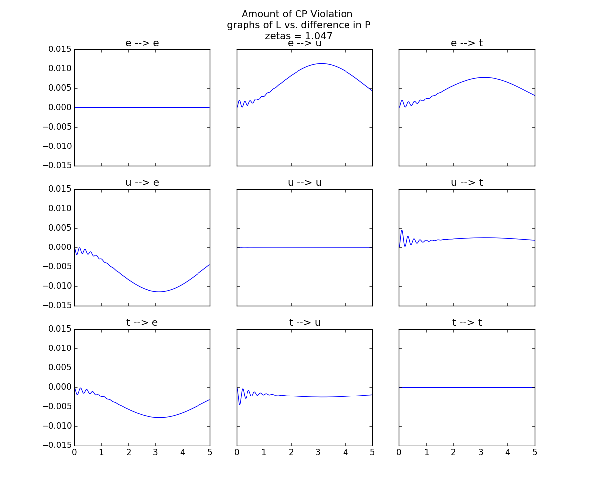
a1=1, a2=2, a3=31, b1=0, b2=0, b3=3, ζ1=π/3, ζ2=π/3, ζ3=π/3, ε1=.01, ε2=.01, ε3=.01
. Kayla Leonard
. Northwestern REU Student 2015
. Student at University of Texas at Austin