On to Off: Predictions for the Radio Afterglows of Nuetron Star Mergers
By Carlo Esquivia and Prof. Wen-fai Fong

My name is Carlo Esquivia, and I study physics at Hamilton College. Over the summer of 2018, I researched with Professor Wen-fai Fong through the CIERA REU program at Northwestern Unversity in Evanston, IL. This project required prior programming experience and comfort manipulating large data sets. I am most thankful for this project because my advisor and I stressed clear scientific communication from the start, which has inevitably taught me how to design and present figures effectively.
In the following paragraphs I will present my research. If you would like to find out more about me, such as my previous experiences, I have created a section for that that has my resume (08/24/18). If you have any general questions about my research or the experience I had this summer, email me and I'll try to get back to you promptly. Thank you, and I hope you appreciate this work.
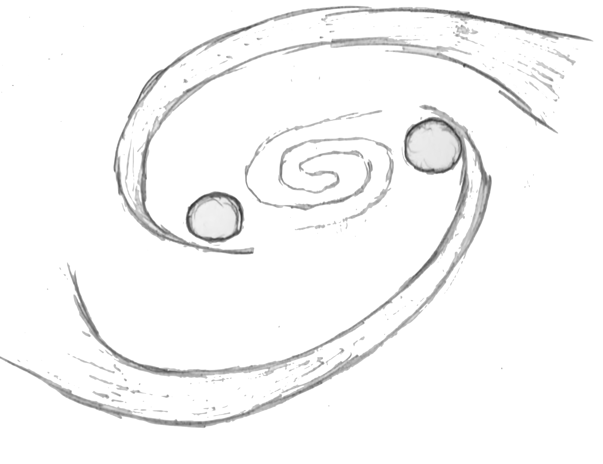
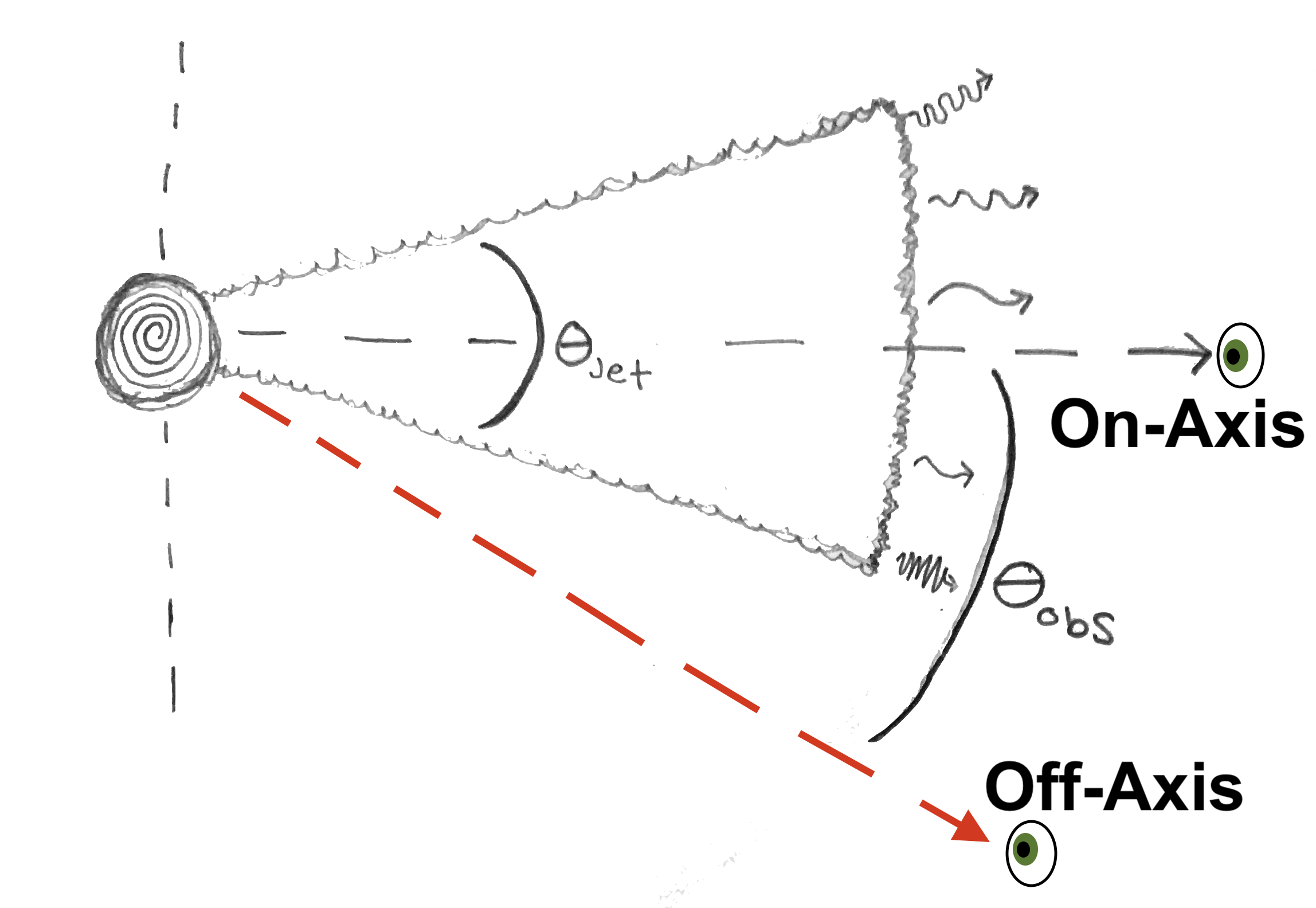
Merging neutron stars form accreting black holes that birth some of the universe's brightest explosions, short gamma-ray bursts (GRBs). The GRB jet interacts with the surrounding medium to produce synchrotron emission called the "afterglow". The afterglow radiates across the electromagnetic (EM) spectrum, producing light at X-ray, optical, and radio wavelengths. Here, we use observations of on-axis short GRBs $(\theta_{obs} = 0)$ to predict the behavior of off-axis afterglows $(\theta_{obs} > 0)$.
Gravitational wave (GW) facilities such as the Laser Interferometer Gravitational-Wave Observatory (LIGO) and Virgo Observatory detect GW emission from neutron star mergers. Since LIGO/Virgo provide poor localizations of ~10-100 of square degrees, we rely on the detection of an EM counterpart (e.g., an off-axis afterglow) to precisely localize the mergers. We use on-axis data to potentially improve searches of off-axis counterparts.
The afterglow depends on two key parameters: the kinetic energy of the material ($E_K$) and the density of the environment (n) with which it interacts. Using data from 39 on-axis short GRBs (Fong et al. 2015), we use the 2D probability distributions in $E_K$ and n as inputs for BOXFIT (van Eerten et al. 2012), which simulates GRBs at various observer angles, $\theta_{obs}$, to compute the light curves of off-axis afterglows. In this project, we assume that the properties of neutron star mergers are drawn from the same distributions as those of on-axis short GRBs.
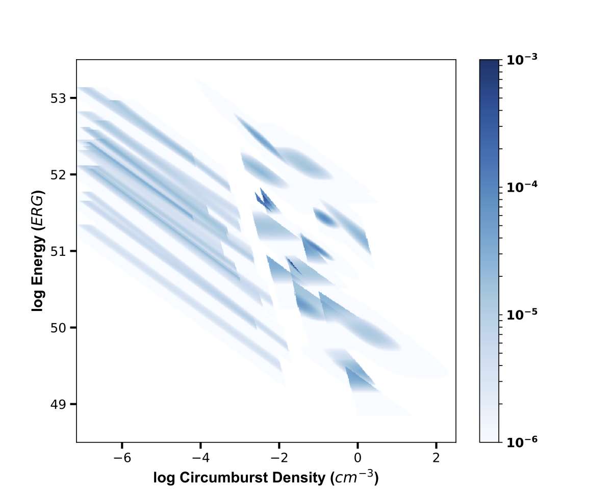
We wrote a set of Python scripts to sum the individual distributions and normalize the result to create a total probability distribution of $E_K$-n from on-axis short GRBs (right). We then performed 2D-sampling of the total distribution, withdrawing 1000 $E_K$-n pairs according to their probability. We used the drawn pairs as parameters for BOXFIT runs, and simulated a $15^{\circ}$ GRB jet at a distance of 200 Mpc and frequency of 10 GHz for three values of $\theta_{obs}$: $10^{\circ}$, $30^{\circ}$, and $60^{\circ}$ (1000 runs each). We created a set of bash scripts to run the simulations on Quest, Northwestern's High Performance Computing cluster. Each simulation took six minutes with 30 processors or greater than four days for 1000 serial simulations. By parallelizing the process, we were able to finish 3000 simulations in under six hours.
We used BOXFIT to generate 1000 light curves each at 10 GHz for $\theta_{obs}$: $10^{\circ}$ (yellow), $30^{\circ}$ (blue), and $60^{\circ}$ (green) from our sampled energies and densities. These are plotted in the figures as flux density versus time (far right). The time axis ranges from a few hours to 10,000 days. Darker regions indicate a higher density of light curves.
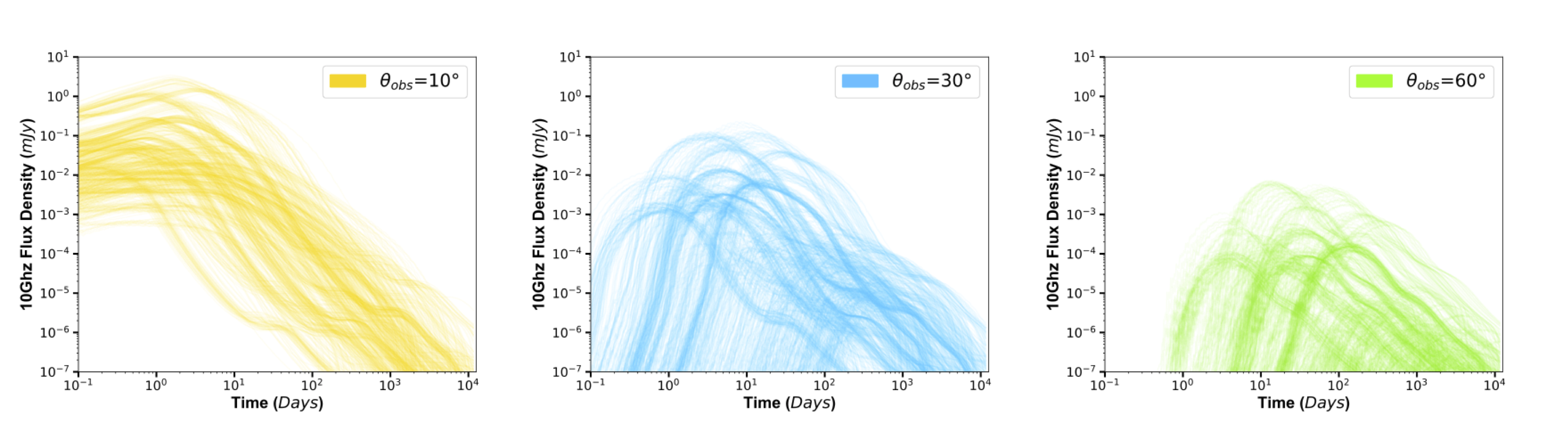
As expected for a nearly on-axis afterglow, the light curves are brightest when $\theta_{obs} = 10^{\circ}$ and have an initial range from $10^{-3}-10^{0}$ mJy. Furthermore, the rate of decay roughly follows a power-law, and the average light curve peaks between 1 and 10 days. Conversely, when $\theta_{obs} = 60^{\circ}$, the light curves are significantly less bright with the maximum flux density being $10^{-2}$ mJy. In addition, the peak timescales span a significantly broader range, between 5-200 days. As expected of an off-axis orientation, they take more time to reach a maximum as the jet comes into view.
The light curves for $\theta_{obs} = 30^{\circ}$ also have a broad range of peak timescales, 1-100 days. Compared to the $60^{\circ}$ light curves, the $30^{\circ}$ light curves on average peak sooner, and reach a higher maximum flux density of ~0.1 mJy. Therefore, the $30^{\circ}$ light curves are as expected for a moderate observer angle. Overall, the light curves demonstrate that when we incorporate the distributions of energies and densities from short GRBs, there is a large diversity in expected light curve behavior.
Since our results are given in flux and time, we aim to answer the following questions: how quickly should we begin observations, and how sensitive should our observations be? Our analysis is geared towards providing observers with information that will directly improve their probability of detection. We have considered that most current radio facilities can achieve limits of ~1 mJy, while the most sensitive facilities at GHz frequencies (e.g., the Very Large Array) can reach achieve ~$10^{-2}$ mJy, and future facilities such as the SKA may reach ~$10^{-4}$ mJy. Our analysis uses these flux limits to show what we can detect based on current and future capabilities. Our tools are interactive and allow the user to query their choice of limiting flux density, $F_{lim}$, and fixed time, t.
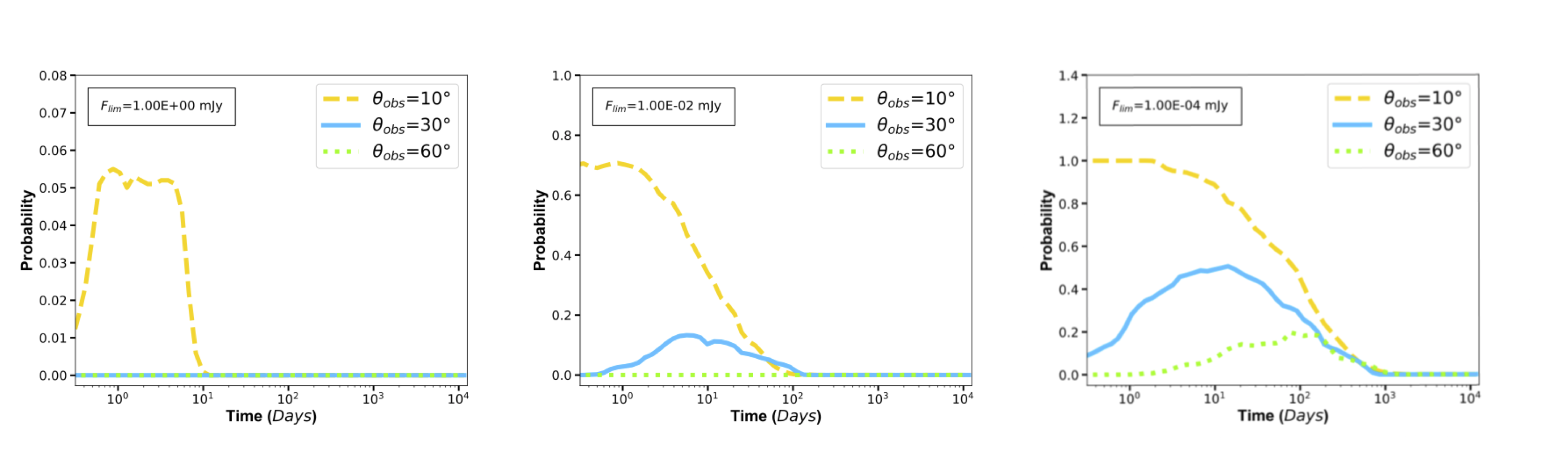
Above, we show the probability of detection for a given limiting flux density, $F_{lim}$, at all times. At $F_{lim}=1.0$ mJy, most radio facilities detect near on-axis GRBs; but at $\theta_{obs}=10^{\circ}$, the probability of detection is ~5%. At $F_{lim}=10^{-4}$ mJy, the probability of detection is greater than 60% at 1 day for $\theta_{obs}=10^{\circ}$, whereas it is about 20% at 10 days for $\theta_{obs}=30^{\circ}$. We show that even our most sensitive facilities cannot detect far off-axis GRBs such as $\theta_{obs}=60^{\circ}$. However, at $F_{lim}=10^{-4}$ mJy, the probability of detection is about 20% at 100 days for $\theta_{obs}=60^{\circ}$. Clearly, our probability of detection saturates at higher sensitivities; for example, at $\theta_{obs}=10^{\circ}$ and $F_{lim}=10^{-4}$ mJy, the probability has saturated. Therefore, there is a need for more sensitive telescope in order to make more observations.
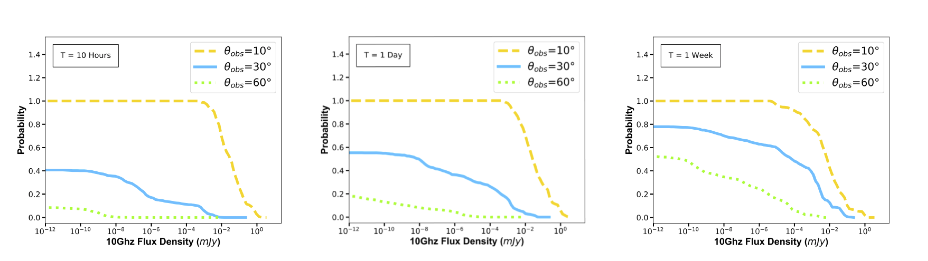
Above, we show the probability of detection versus limiting flux for a series of three fixed times: t = 10 hr, 1 day and 1 week. These figures allow us to visualize the flux limits for when every off-axis observation saturates to their highest probability of detection. These points of saturation remain the same for every time, but the probability of detection at those points change as a function of time. For instance, at $\theta_{obs}=10^{\circ}$, the turning point of saturation varies from 1 day to 1 week, but the overall shape is maintained. Likewise, for $\theta_{obs}=30^{\circ}$, the probability increases from 1 day to 1 week because a higher percentage of light curves are found at later times at off-axis observations. These figures are useful because they show the critical role timing plays in our observations, as well as the limited return of deeper observations past a certain depth.
Current predictions to locate GRBs within large gravitational wave localization regions have not relied on actual observations to detect off-axis GRBs. Using BOXFIT, we used on-axis GRBs to simulate light curves of off-axis afterglows for varying $\theta_{obs}$. These light curves confirmed our expectations of how off-axis observations behave such as a difference in brightness, shape, and rate of decay.
We have created a tool for others that is easily adaptable to their own observational data. The process of sampling and changing parameters can be adopted to work for other models that require similar inputs. In addition, the light curve analysis can be modified and extended beyond our current needs. We plan to develop a working graphical interface and repeat our measurements for other $\theta_{obs}$, frequencies, and limits. This is simply the beginning in our endeavors to use on-axis observations of short GRBs to improve our expectations and searches of off-axis GRB afterglows. This will help not only for GW events, but also in predicting rates in future untargeted surveys such as LSST.
Fong et al. 2015, ApJ, 815, 102
van Eerten et al. 2012, ApJ, 749, 44
This material is based upon work supported by the National Science Foundation under Grant No. AST-1757792. Any opinions, findings, and conclusions or recommendations expressed in this material are those of the author(s) and do not necessarily reflect the views of the National Science Foundation.
This research was supported in part through the computational resources and staff contributions provided for the Quest high performance computing facility at Northwestern University which is jointly supported by the Office of the Provost, the Office for Research, and Northwestern University Information Technology.