

A Fast Method to
Predict Distributions of
Binary Black Hole Masses
Based on Gaussian Process Regression
A Fast Method to Predict Distributions of Binary Black Hole Masses Based of Gaussian Process Regression
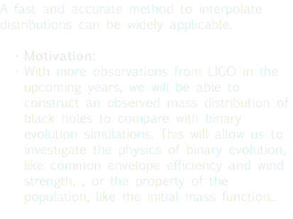
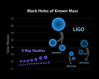
Introduction
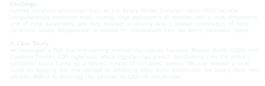
Case Study Data
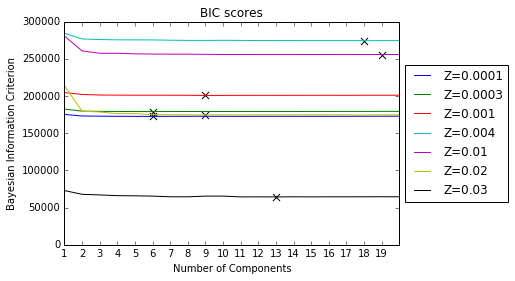
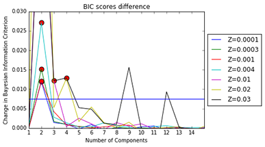
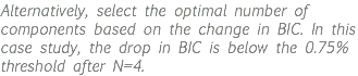
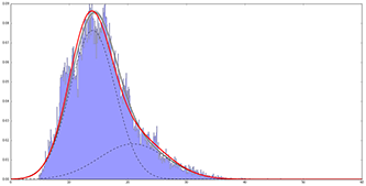
Quantify a Distribution: Gaussian Mixture Model


Gaussian Mixture Model with 2 Components
Z=0.0001
Gaussian Mixture Model with 3 Components
Z=0.0001
Gaussian Mixture Model with 2 Components
Z=0.0003
Gaussian Mixture Model with 2 Components
Z=0.001
Gaussian Mixture Model with 2 Components
Z=0.004
Gaussian Mixture Model with 2 Components
Z=0.01
Gaussian Mixture Model with 2 Components
Z=0.02
Gaussian Mixture Model with Components
Z=0.03
<
>

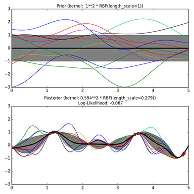
Interpolate Parameters: Gaussian Process


GP with linear scale
GP with linear scale
GP with linear scale
GP with linear scale
GP with linear scale
GP with linear scale
<
>


GP with semi-log scale
GP with semi-log scale
GP with semi-log scale
GP with semi-log scale
GP with semi-log scale
GP with semi-log scale
<
>
Reconstruct Distributions


Construct the predicted distribution based on estimated parameters using four methods
Construct the predicted distribution based on estimated parameters using four methods
Construct the predicted distribution based on estimated parameters using four methods
Construct the predicted distribution based on estimated parameters using four methods
Construct the predicted distribution based on estimated parameters using four methods
<
>
Model Evaluation


Future Prospects
![This is an ongoing project and there are many possible improvements as well as new opportunities to apply this method. • Modify Gaussian Mixture Model: • Instead of assuming the distribution is a Gaussian mixture, we can use instead Voigt profiles or gamma distributions to count for the long tails in our data histograms. • Improve on Gaussian Process: • The current method of GP does not take into account that covariance of a Gaussian component should always be non-negative and the weight of it should be within [0,1] interval. That has resulted in negative covariance and weight predictions. Restrictions on the range of GP priors may fix the problem. • Investigate other parameters: • Instead of looking at metallicity, we can run binary stellar evolution for other parameters, which will give us a denser dataset and enable us to perform higher-dimensional analysis.](images/u1793-25.png?crc=120111002)