Project Description
Now that the Laser Interferometer Gravitational Wave Observatory (LIGO) has detected gravitational waves (GWs) from binary black hole mergers, it is expected that GWs from binary neutron stars (BNSs) and neutron star-black hole (NSBH) binaries will be detected in the near future. Along with GWs, these systems are thought to produce electromagnitic (EM) signals such as short gamma-ray bursts (SGRBs) and kilonovae. SGRBs occur on the order of milliseconds, with afterglows that can last as long as several days, and are visible in the optical band ( Metzger & Berger (2012)). Kilonovae on the other hand, are expected to last as long as several days to a week, and are anticipated to be observable in the optical to near-infrared range ( Metzger (2017)).
Using fit formulas for NSBH and BNS ejecta mass, developed by Kawaguchi et. al (2016) and Dietrich & Ujevic (2017) respectively, we can calculate the ejecta mass of a number of events, assuming different EOSs. Then for each event, we can calculate kilonova light cuves.
Nuclear Equation of State
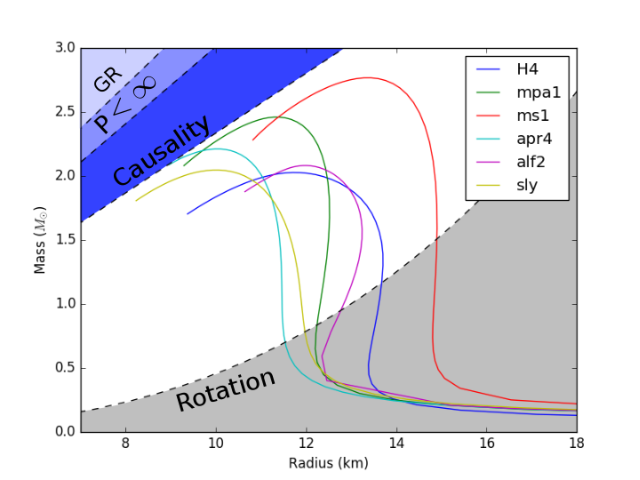
A nuclear equation of state (EOS) in the context of neutron stars (NSs), in simplest terms, describes how "squishy" NSs are. In more technical terms, an EOS describes the internal pressure ($p$) of a NS as a function of both energy density ($\epsilon$) and baryonic mass density ($\rho$). By integrating an equation, known as the Tolman-Oppenheimer-Volkoff (TOV) equation, which describes NSs in hydrostatic equilibrium, one can determine the mass and radius of a NS for a specific EOS given a central density. If this equation is integrated for a range of central densities, one can generate a mass-radius curve for an EOS (see Figure 1).
In this study, we use six different EOSs: ALF2, APR4, H4, MS1, MPA1, and SLy. These were chosen from the set of EOSs used in J. Read et. al. (2008) In the future, we plan to include more EOSs in our study, but for now we limited our attention to six of the more common EOSs. None of the EOSs we consider include any exotic matter.
Events Population
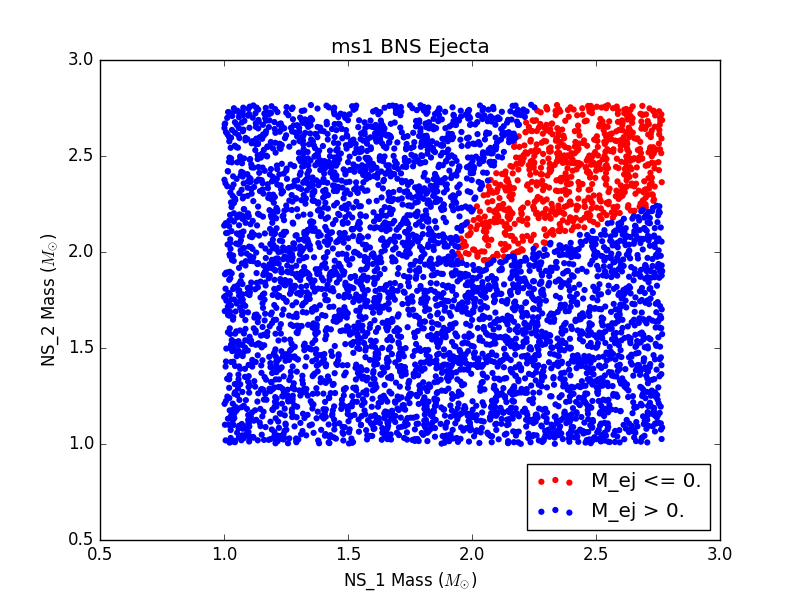
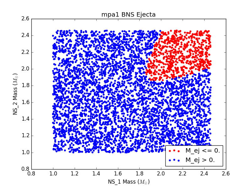
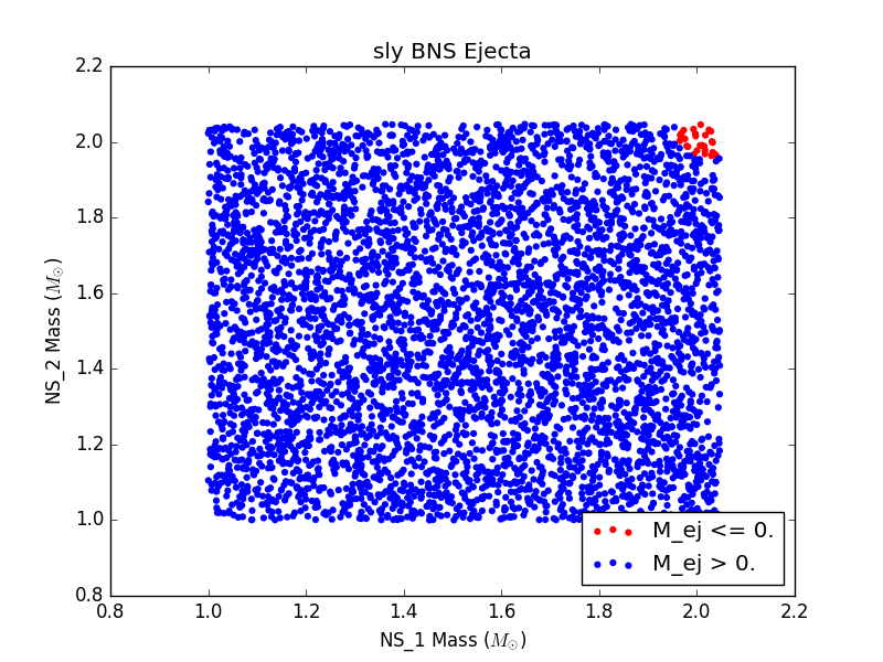
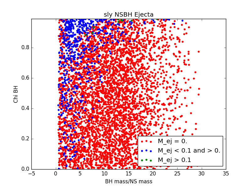
For each EOS, we generated a population of binary neutron stars (BNSs) and neutron star-black holes (NSBHs). We ensured that for every event in our populations, the binary merger had 1) a detectable gravitational wave (GW) signal and 2) a visible electomagnetic (EM) counterpart. For GW detectability, we require a miniumum signal to noise ratio of 5.5 in at least two detectors. For EM counterpart visibility, we require that ejecta mass be nonzero. We assume a GW detector network of LIGO Livingston, LIGO Hanford, and VIRGO.
BNS Events
BNS specific parameters and ranges include:
- $M_{NS}$: 1-Max $M_{\odot}$
- $R_{NS}$: Determined by EOS
- $M^*_{NS}$: Determined by EOS
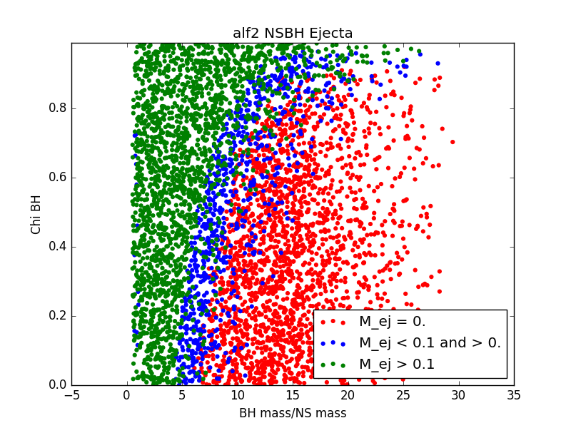
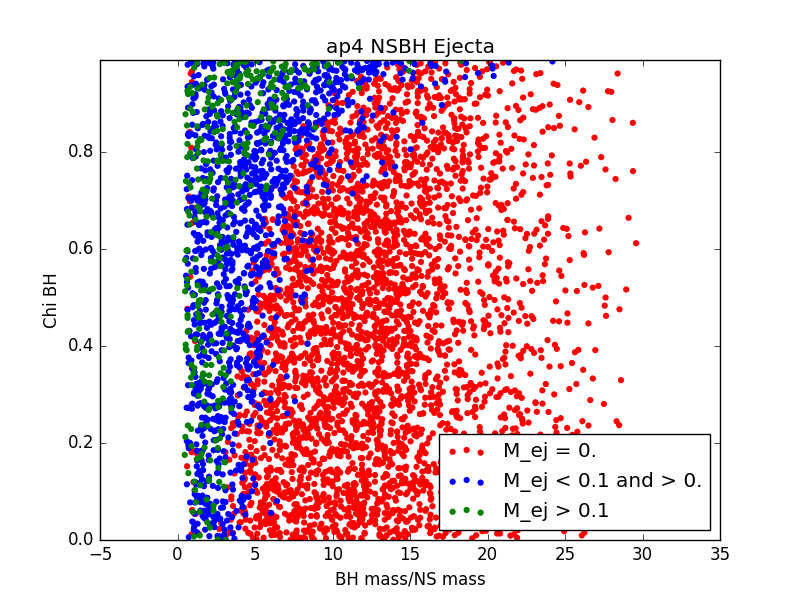
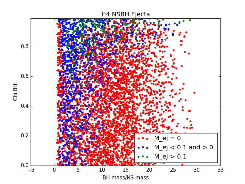
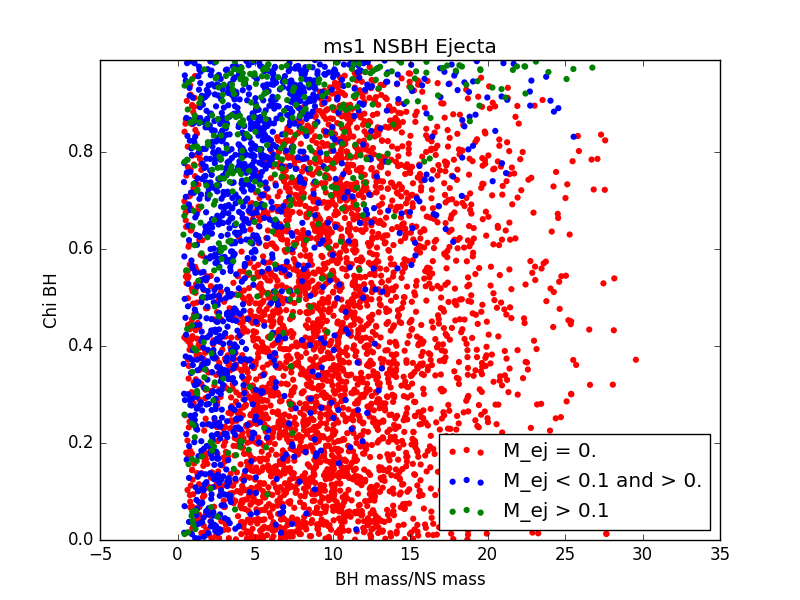
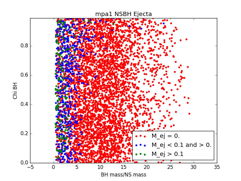
NSBH Events
NSBH specific parameters and ranges include:
- $M_{NS}$: 1-Max $M_{\odot}$
- $R_{NS}$: Determined by EOS
- $M^*_{NS}$: Determined by EOS
- $M_{BH}$: 3-50 $M_{\odot}$
- $\chi_{BH}$: 0-1
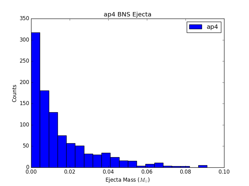
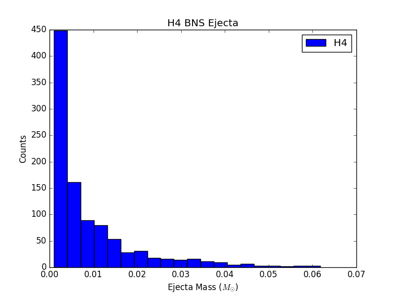
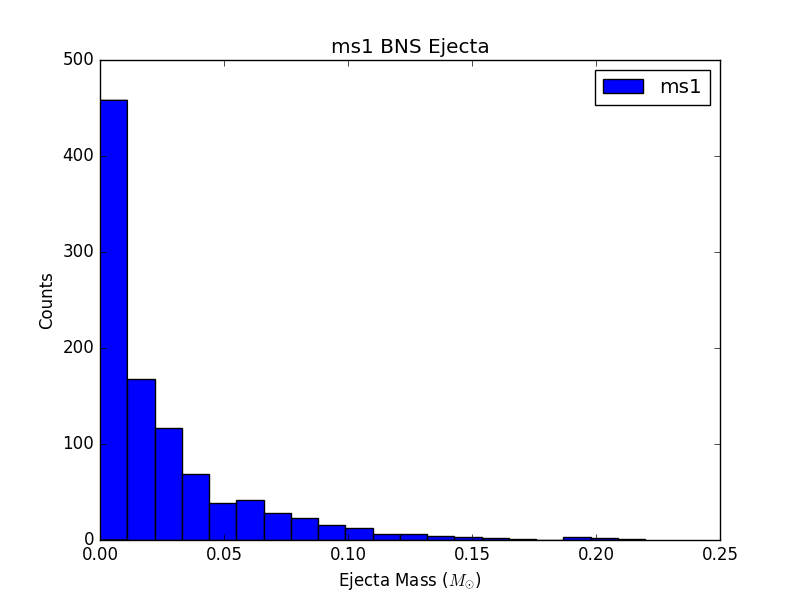
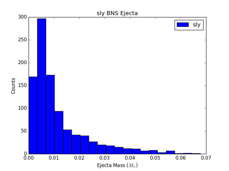
Ejecta Mass Distributions
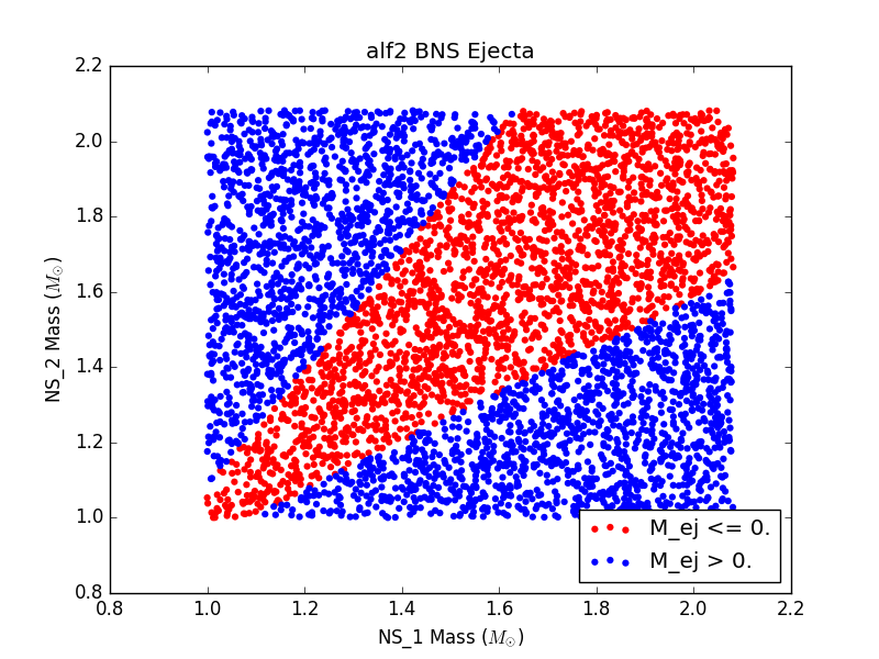
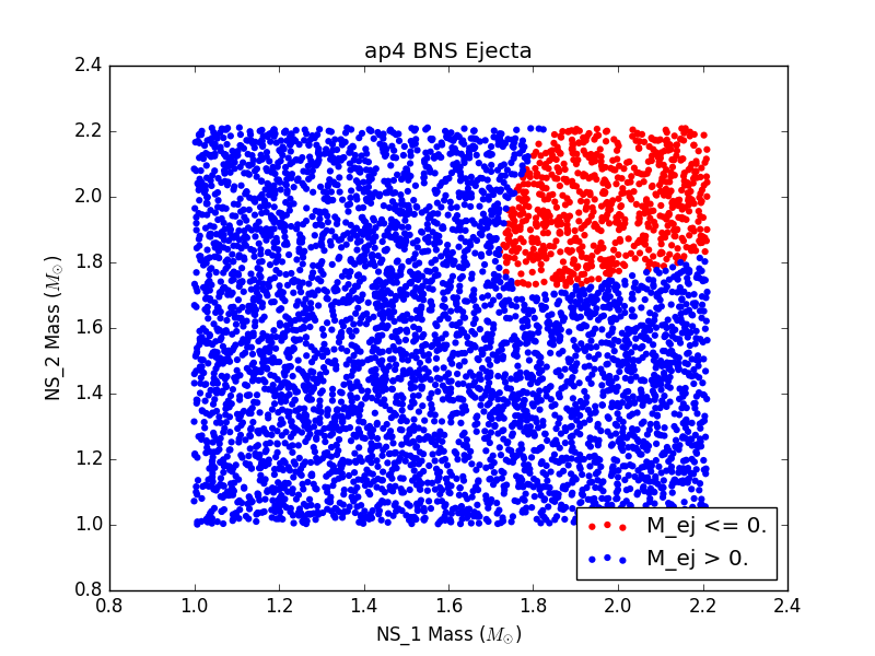
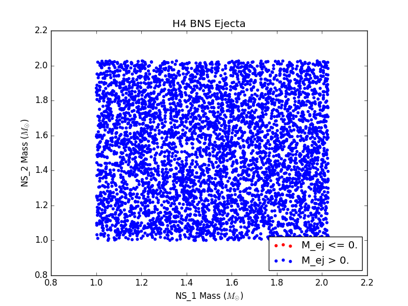
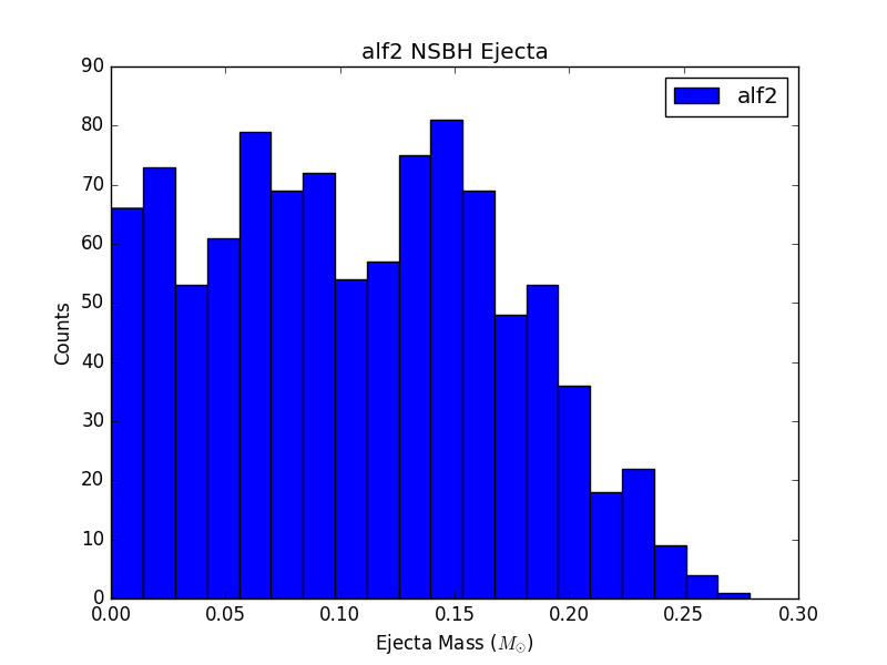
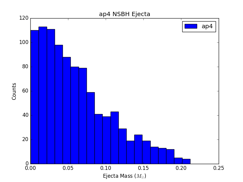
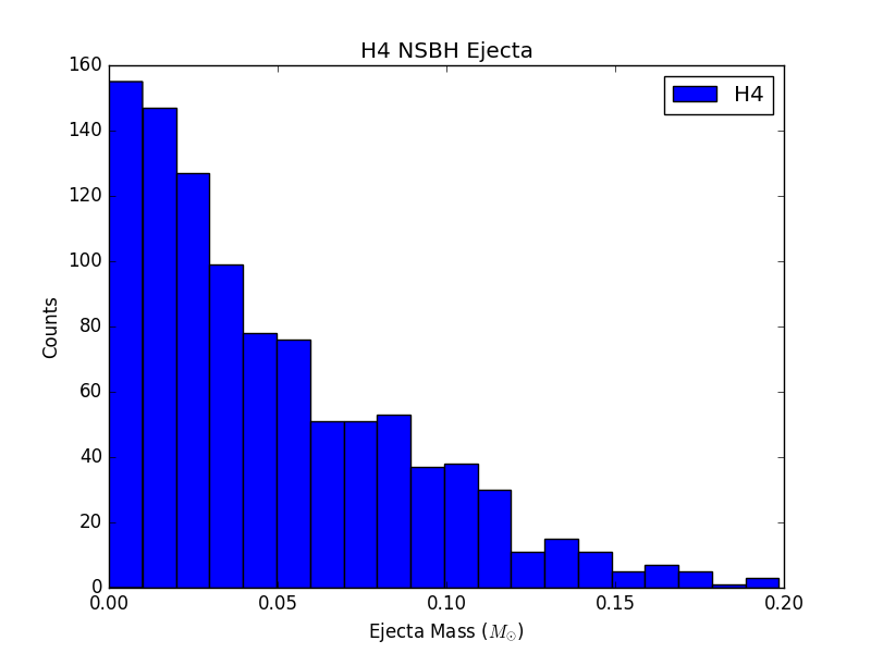
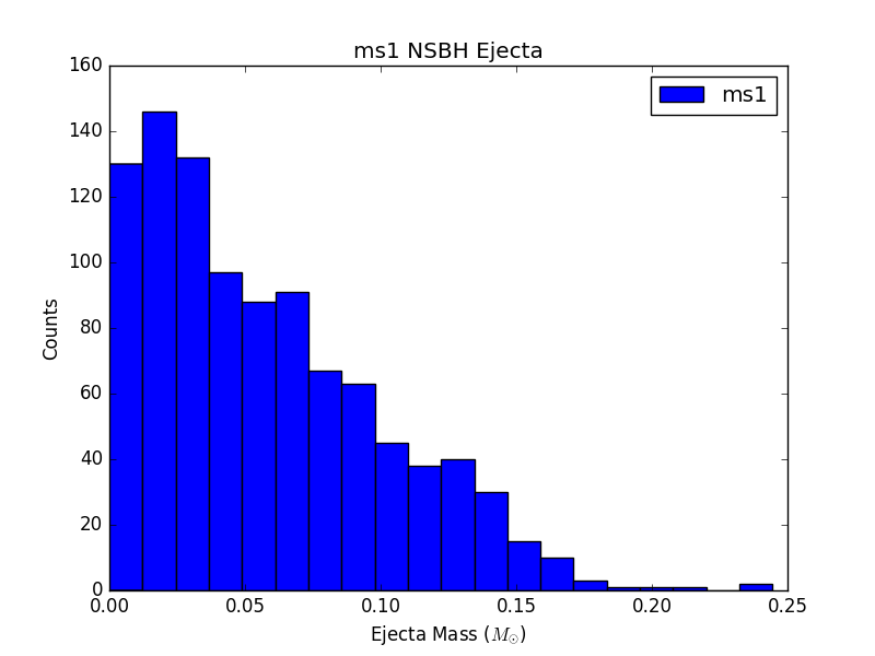
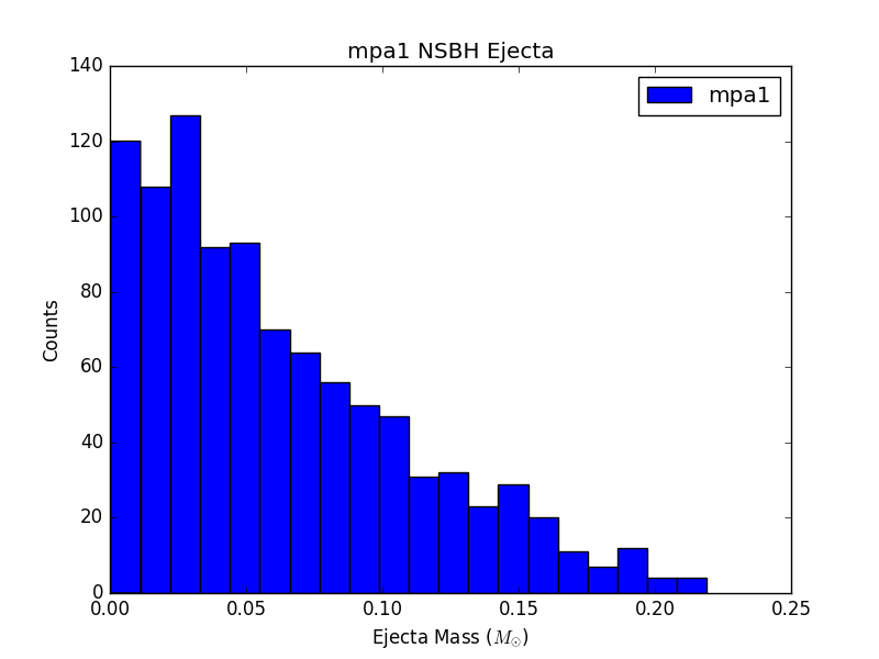
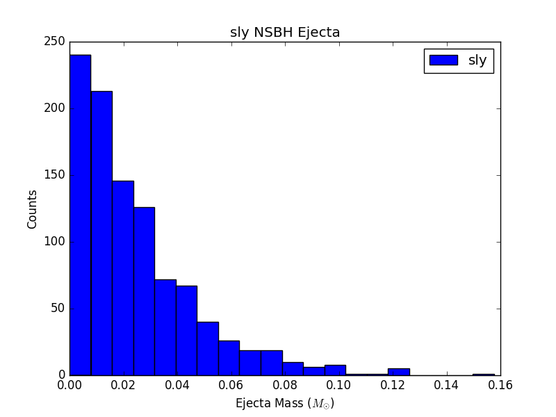
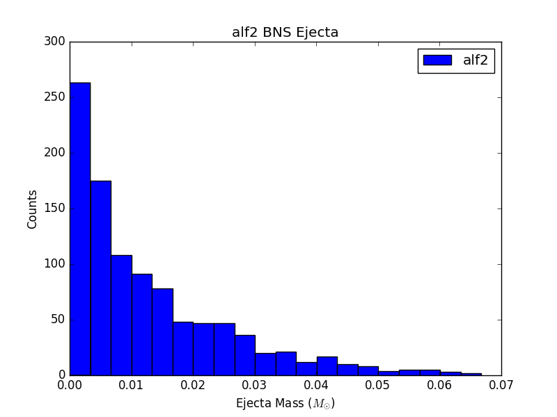
For 6 populations of 1000 NSBH and BNS sources, each assuming a different EOS, histograms of ejecta mass are not largely distinguishable (see Figure 3). This could be due to populations that are not large enough, or could just be a result of the fact that the parameter space being sampled is so large, and potential differences are getting washed out.
Kilonova Light Curves
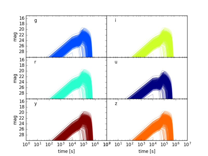
Kilonovae are a result of the radioactive decay of nuclear matter torn off of NSs in the violent mergers of BNS and NSBH systems. The duration and magnitude of kilonovae depend on both the amount and the velocity of the ejecta. The timescale of kilonova light curves can be described by:
$t_{peak} \approx 1.6d \bigg(\frac{M}{10^{-2}M_{\odot}}\bigg)^{1/2}\bigg(\frac{v}{0.1c}\bigg)^{-1/2}\bigg(\frac{\kappa}{1cm^{2}g^{-1}}\bigg)^{1/2}$
according to Metzger (2017). Using equations adapted from B. Metzger's Kilonova Handbook (2017) we can use the ejecta mass we calculate to generate light curves (see Figure 4).
Note: The authors of both the NSBH and BNS ejecta formula papers have created online calculators for generating light cuves assuming certain initial event parameters. The one for NSBH can be found here and the one for BNS here.
Going Forward
Once we have thoroughly tested this model for GW localization, ejecta calculation, and light curve generation, we can apply it using more EOSs and different detector configurations. We can then draw some conclusions about the plausibility of detecting a GW signal and an EM counterpart. Eventually, when GW detections from NSBH and BNS are made, we may be able to apply our model in order to place some constraints on possible NS EOSs.