The Kuramoto Model as Motivator

The Kuramoto model is a nonlinear differential equation that relates the frequency of, or rate of change in, an oscillation to the current position in the oscillation cycle. What is this "oscillation?" It can be many things. Some examples include:

• Blinking of certain firefly species
• The mechanical ticking of a metrnonome
• Steps of people in a crowd walking on an unstable bridge

Mathematics of the Kuramoto model

The Kuramoto equation is customarily written as follows:

$\frac{d\theta_i}{dt} = \omega_i + \frac{K}{N}\sum_{j=1}^{N}\sin(\theta_j - \theta_i)$

The components contributing to the rate of change are stated in the right hand side of the equation.

• $\omega$: the object's natural frequency--the normal speed at which it will perform its cycle, absent driving or dampening forces.
• summation term: an adjustment to the the frequency that results from forces between the object and all the other objects in the system.

The variables in the system are further defined as below.

• K: a constant representing the strength of the coupling (how strongly the objects affect each other).
• N: the number of objects in the system
• $\theta$: the current phase of the object, that is, where it is in its cycle.

The subscript i denotes a specific object in the system. This means that every object in the system will have its behavior described by this equation. The subscript j varies between 1 and N and designates "other" objects: this is where the summation comes in. The object's natural frequency is adjusted up or down depending on its position relative to another object in the system. The the fact that the difference occurs inside of a sine function indicates that the sign of the adjustment will change depending on whether the jth object is ahead or behind the current object i.

Visualization of behavior

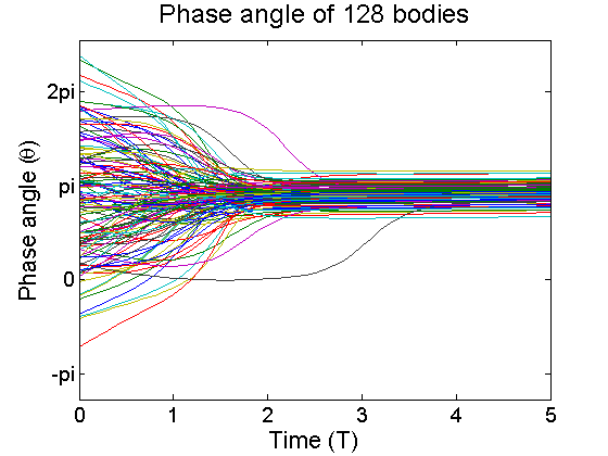
So, what does this say about the system? The upshot is that if the coupling strength K is high enough, objects in the system--no matter if they are living creatures or inanimate objects--will adjust their cycles to match their neighbors! When plotted, this behavior creates intricately and chaotically overlapping paths before synchronization, as shown at left.

In the plot of the phase of oscillators over time, each colored line represents a different object in the system, with its own unique natural frequency. At the beginning of the simulation (or, in real life, when the objects start oscillating), all objects start at a given point in their cycle. But over time, minor adjustments to their frequencies occur due to effects from the others surrounding them. The end result is that all the objects coalesce to a common phase, which is synchronization.

If we envision the objects as particles on a circular track (for example, the unit circle), the objects will all be clustered around the phase angle of synchronization and will move around the circle together, like a group of runners in a race who are neck and neck.

We can use the fact that the objects are all at very slightly different radii around the circle to describe the degree of synchrony. By performing a vector sum of the components of the radius of each object, we obtain components for an "average" radius of all the oscillators. The maximum of this radius will be the radius of the circular track. When this maximum is equal to the "average" radius, complete synchrony is achieved. The radius approaching 0 would correspond to a state in which the objects are randomly distributed about the circle--i.e., the beginning of the simulation, when they are all at different phases. An animation illustrating this idea follows (Source: Wikipedia, credit to Stewart Heitmann).

Fireflies

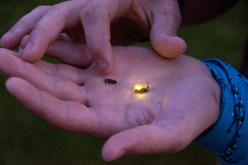
The canonical example of this mathematical model is the blinking of certain firefly species, specifically Pteroptyx malaccae and Pteroptyx cribellata.

Image credit: Lightning bugs in York, PA, Flickr user tom.arthur, 2009