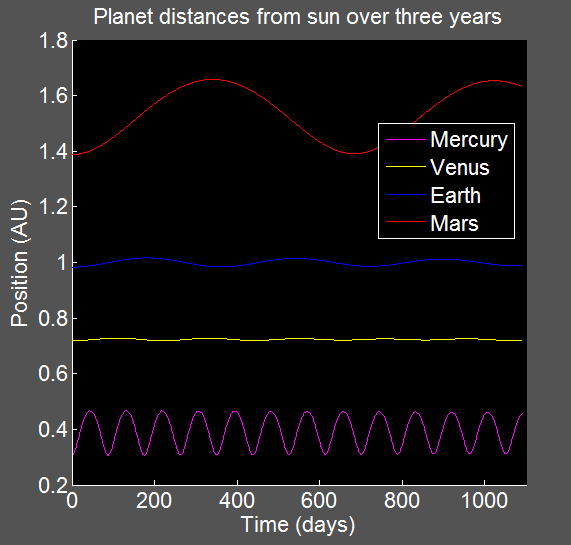
With the completion of the basic N-body simulator without collision handling, a fairly simple simulation of the orbits of the 8 planets can be run as proof of concept. The simulation tracks the distance of each planet from the sun over time, with each planet's total distance oscillating about its mean. The plot at left shows an example of the results of this simulation (with distances in astronomical units) over a time span of three years. Note that for this particular simulation, all 8 planets and the sun were simulated, but only the four inner planets are plotted as the significant increase in distance of the outer planets would relegate all the inner planets to a very narrow region at the bottom of the plot.

An alternative, and perhaps more attractive, method for visualization of the data is with animation--especially since the simulation concerns bodies moving through space. Animation for the N-body simulation will be completed after further optimization and extension of the main features of the code. An example animation for a two-body system, the sun and the Earth, is shown at right.

Collision handling

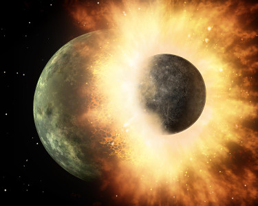
In order to simulate interactions of bodies in close proximity, such as those in a circumplanetary dust disk, the code must handle collisions. This allows simulations of larger N and at closer distances to a central body (for instance, distance < 1 AU). In the original simulation without collision handling, collisions would result in division by zero errors as d → 0. The collision is assumed to be inelastic; therefore the energy of the two-particle system is reduced by some fractional amount after the collision and the remaining energy is randomly distributed between the two bodies within a certain range. The range is required as decreasing or increasing a velocity by too much would violate conservation of momentum.

Our collision handling can be outlined as such:

1. A condition is set for what constitutes collision--1000 km is initially used to speed debugging and ensure collisions actually occur, since the orbits are over very large distances.
2. During integration, we use ode45's options and odeset to configure an event function that checks for collisions at every step.
3. In the event of a collision, integration is stopped and the following occurs:
1. The code calls another function whose job is to solve a system of equations for the final velocities of each body. The system is defined by conservation of momentum along all axes, dissipation of energy and division of the remaining total energy to each of the two bodies using a random fractional value within a certain range.
2. Using solution, the velocities for each body are inserted into a new set of initial conditions for all the objects in the system.
3. Integration is restarted using the new initial conditions, picking up from the time step where it previously left off.

Allowing changes in velocity as described enables the bodies to alter the radius of their orbits around the central body. Lower orbits indicate higher kinetic energy of the body, while higher orbits indicate lower kinetic energy. The effect is that the bodies will speed up or slow down as a result of the collision--similar to the way that bodies obeying the Kuramoto model will alter their frequencies according to the presence of neighbors.

Custom nonlinear model of force interactions

We are currently working to adapt the code to use a new differential equation for the changes in orbital speed of a collection of many bodies around a much larger body—for example, a dust ring around a planet. This equation will be reminiscent of the Kuramoto model:

$\frac{d\theta_i}{dt} = \omega_i + \frac{GK}{4R^3} \int_0^{2\pi} \frac{\rho (\theta ')d\theta '}{\sin^2(0.5|\theta-\theta '|)}$

Like the basic Kuramoto model, this equation expresses the idea that the frequency of an oscillator is modified from its natural frequency by a term comprised of effects from all other oscillators in the system. In this case, when N will be very large, the sum can be approximated with an integral. R represents the radius to the orbited body, G is the gravitational constant, K is a scaling constant and $\rho$ is the density of material in the disk.