SFR Indicators

Understanding the SFR of galaxies is of major importance when seeking to understand how galaxies form. In regions like the Milky Way one can count objects or events forming new stars in order to derive an SFR from that region Chomiuk and Povich (2011) and in other regions one can use SFR indicators to measure the luminosity over some wavelength (Calzetti 2013). Over the past decades SFR indicators have been calibrated with the goal to identify newly formed stars through multiple emissions (Calzetti 2013). Some of these emissions include emission lines from ionized gas surrounding massive stars, infrared emission lines re-emitted by interstellar dust, x-ray emissions dominated by x-ray binaries, emissions dominated by the radio continuum and UV continuum measurements (Kennicutt and Evans 2012). A traditional method relates the SFR of a galaxy to be proportional to the luminosity by assuming a constant SFR for a certain time interval (Buat et al. (2012) , Kennicutt and Evans (2012)).

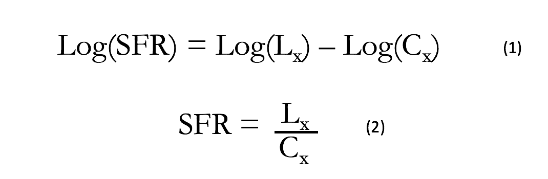
Equation 1 shows the logarithmic SFR can be acquired by taking the difference between the logarithmic luminosity and logarithmic calibration constant. Equation 2 shows a simplified version on Equation 1. The calibration constant arises from the assumption of a constant SFR in order to make the SFR proportional to the luminosity. Each calibration constant is unique to the specific band used to probe the SFR. Two of the SFR indicators we are interested are derived from Far Ultra Violet (FUV) continuum spectrum and Hα emissions shown in Table 1 below. The table also shows the units for the luminosities needed for a specific calibration constant.

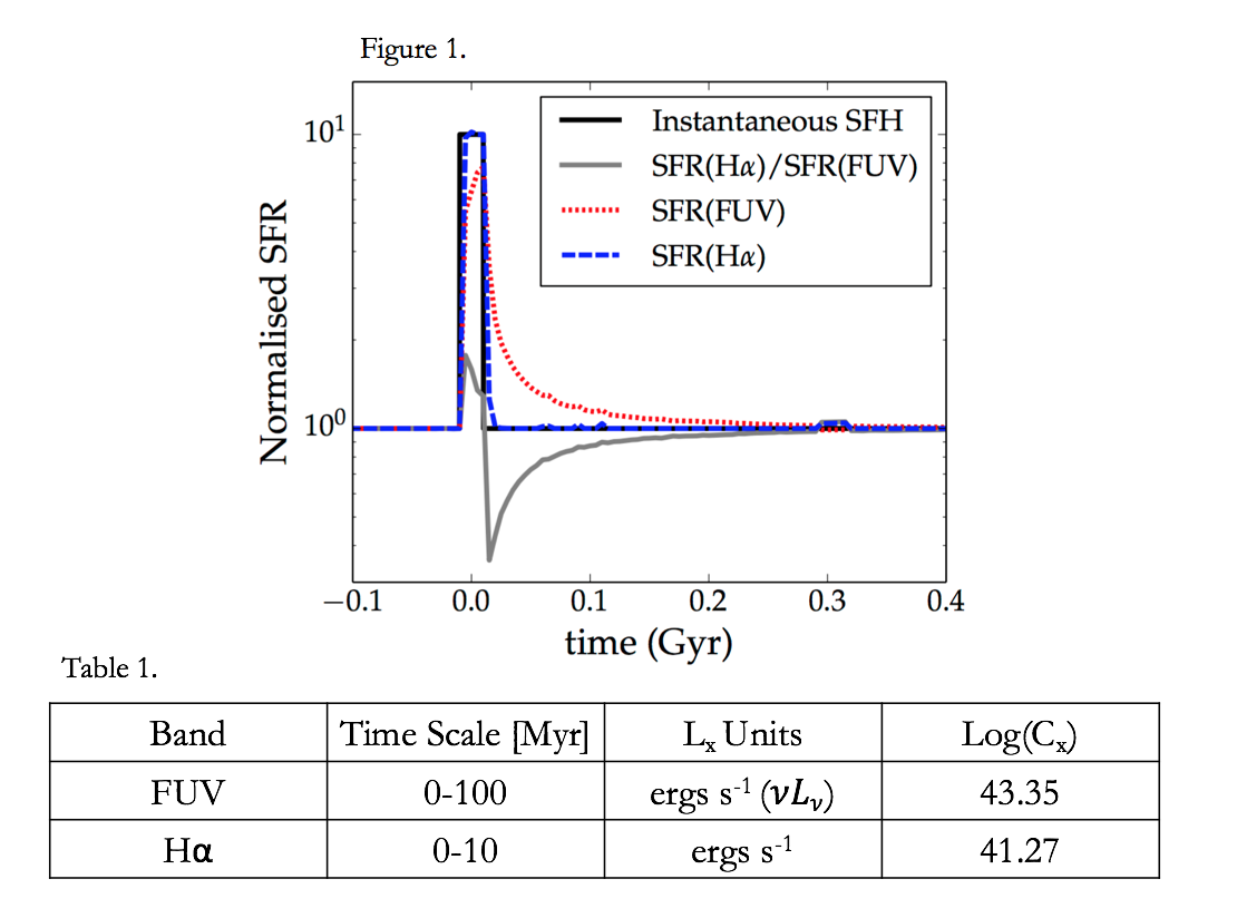
In our work, the two indicators used: SFR(Hα) and SFR(FUV) were calculated using the similar prescription as in Sparre et al. (2017). A GALEX-FUV filter is used in the stellar spectra flux calculations for the SFR(FUV) indicator and the SFR(Hα) indicator is assumed to be proportional to the flux of ionizing photons. Far Ultra-Violet (FUV) emissions trace stars formed over the past 100 Myr (Murphy et al. 2011), and those from ionized gas (Hα) trace stars formed in the past 10 Myr (Hao et al. 2011). See Figure 1, Sparre et al. (2017) and Table 1. However, recent galaxy surveys as well as galaxy formation theoretical models yield time variable (bursty) star formation histories (SFHs) which suggests that star formation occurs at different time scales.

Bursty Star Formation Histories

The FIRE simulations predicts that the SFR of galaxies tend to be bursty at higher redshifts (Muratov et al. 2015, Faucher-Giguère 2017 ). Observations like: Shivaei et al. 2015, Guo et al. 2016, and Shimakawa et al. 2017 also suggest bursty star formation. Our project is motivated by the common assumption made when calibrating SFR indicators. It is assumed that the SFR of galaxies remains constant for a period of time which as shown in recent observations and simulations that may not be the case. In this work we use the self-consistent star SFHs realized in the FIRE simulation (Hopkins et al. 2014, 2017) to quantify differences between observationally-inferred SFRs. We use different indicators and true SFRs, as a function of galaxy mass and redshift to also predict time scales that specific SFR indicators are averaged over.

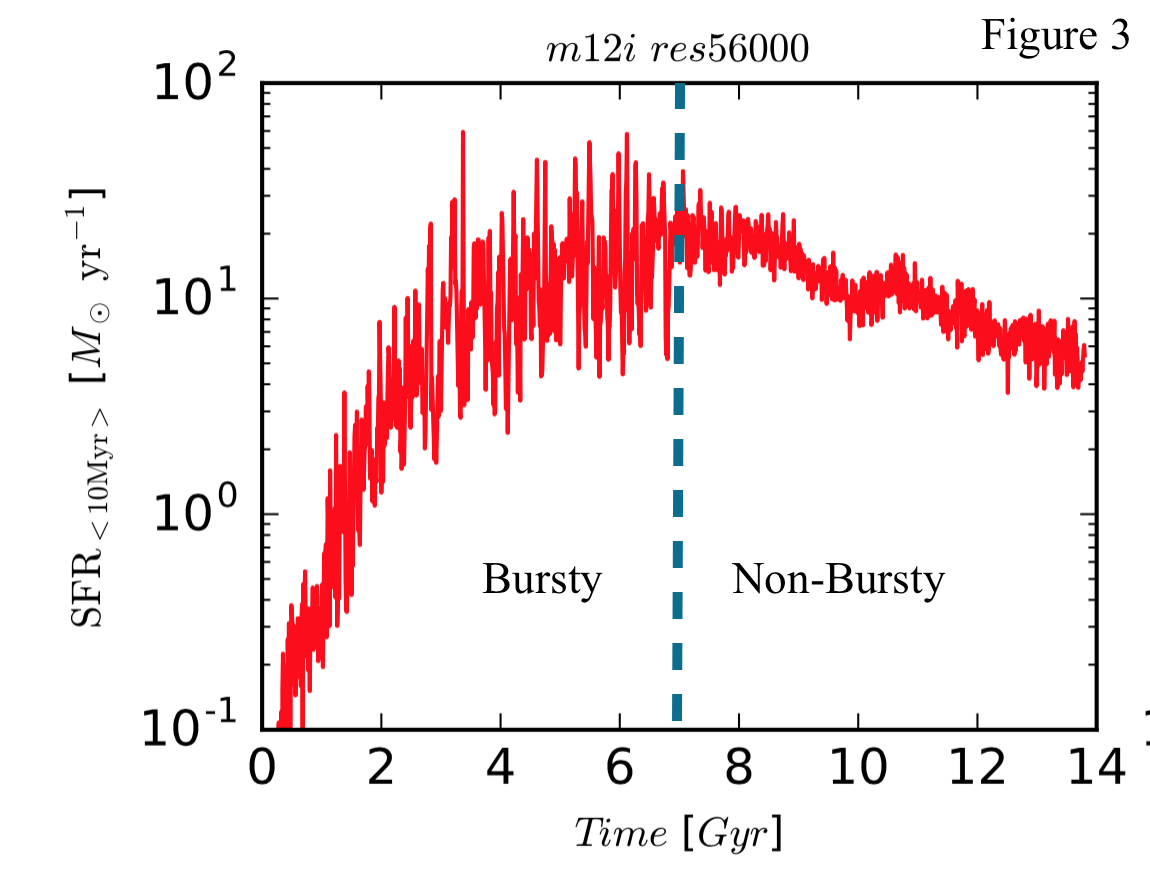
Figure 3. 10 Myr boxcar average SFH of the Milky Way mass-like galaxy -- m12i. We define the bursty SFH of m12i to be at z ≳ 0.7 and the non-bursty regime at z ≲ 0.7.

Reconstruction of Star Formation History

In order to analyze the different SFRs in the FIRE simulations we begin by reconstructing the SFHs of our galaxy simulations. Figure 4 shows m12i at redshift zero where the green boxes enclose some (not all) of the stars as well as dust in the simulation at that time.

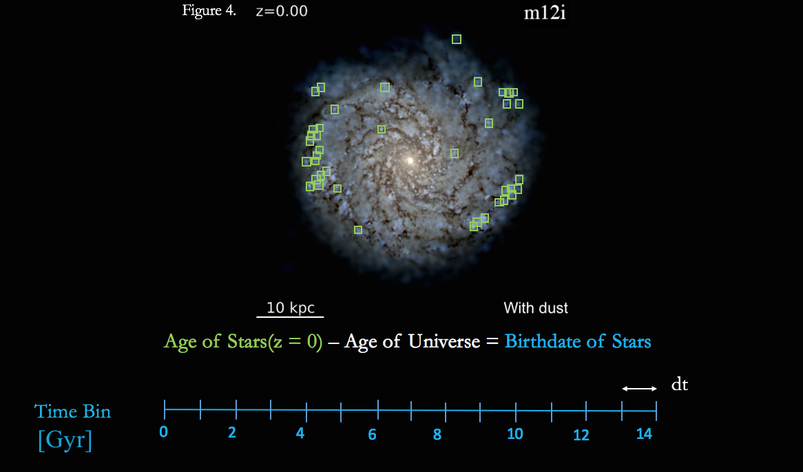
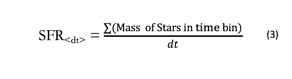
To reconstruct the SFHs of our simulations we determined the ages of each star particle (green) at redshift zero and subtracted their ages from the current age of the universe. By doing so we are able to determine the time at which the stars were born (birthdate of stars). We bin each star particle with their corresponding birthdate and are able to construct a histogram of stellar masses and ages of the star particles in the simulations. The star formation rate is then calculated by taking the sum of stellar masses in each bin and dividing by the time separation of each bin, Equation 3 below. This method of binning serves crucial because it allows us to average our SFHs at different time scales.

Preliminary Results

We average the true SFR of our simulated galaxy over different time scales in order to match the physics of what the observational indicator is doing. The scatter plots in Figure 5 will decrease at an average time scale that most accurately resembles what the indicator is doing. To determine the scatter we determine a best fit line through our SFR data set and calculate the root mean square (RMS) relative error.

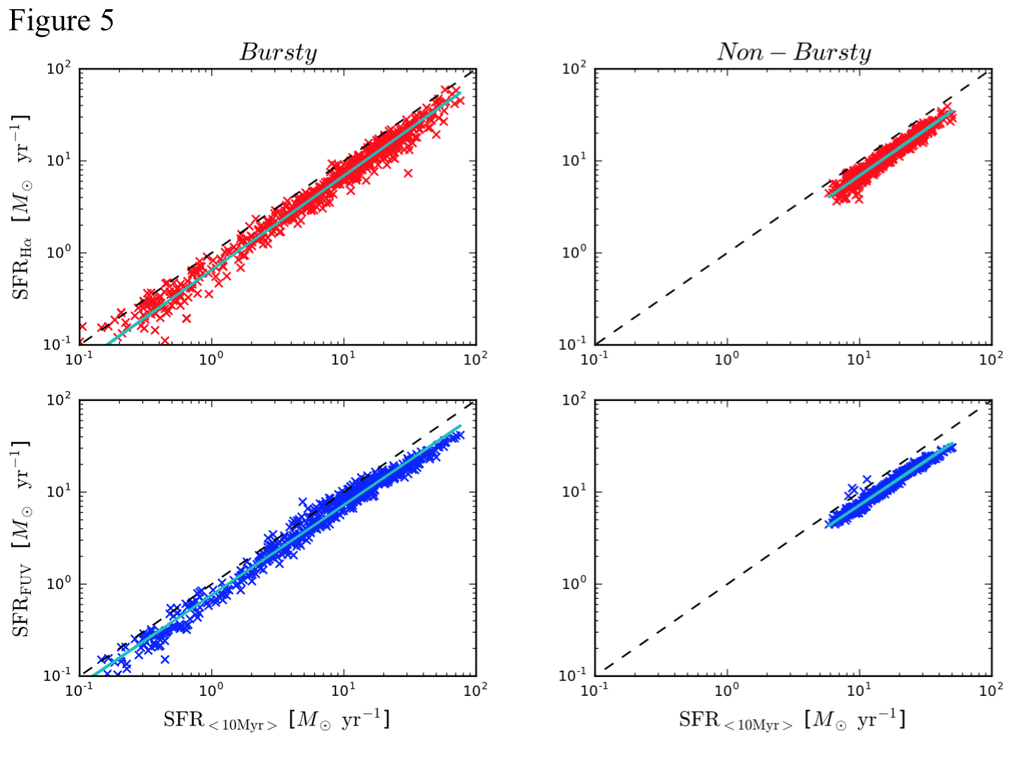
Figure 5. These scatter plots are for m12i. Each point was generated by binning the ages of the stars in the simulation. The SFR of the galaxy (x-axis) has been averaged at a time scale of 10 Myr (dt = 0.01 Gyr). The y-axis on the first row shows the SFR probed by Hα emissions and the y-axis on the second row show the SFR probed by the FUV continuum spectrum. The black dashed line shows a one-to-one correlation and the cyan line is the best fit line between the SFR derived from the indicators and the averaged SFR. The first column of the plot shows the Bursty regime and the second column is the Non-Bursty regime shown in Figure 3.

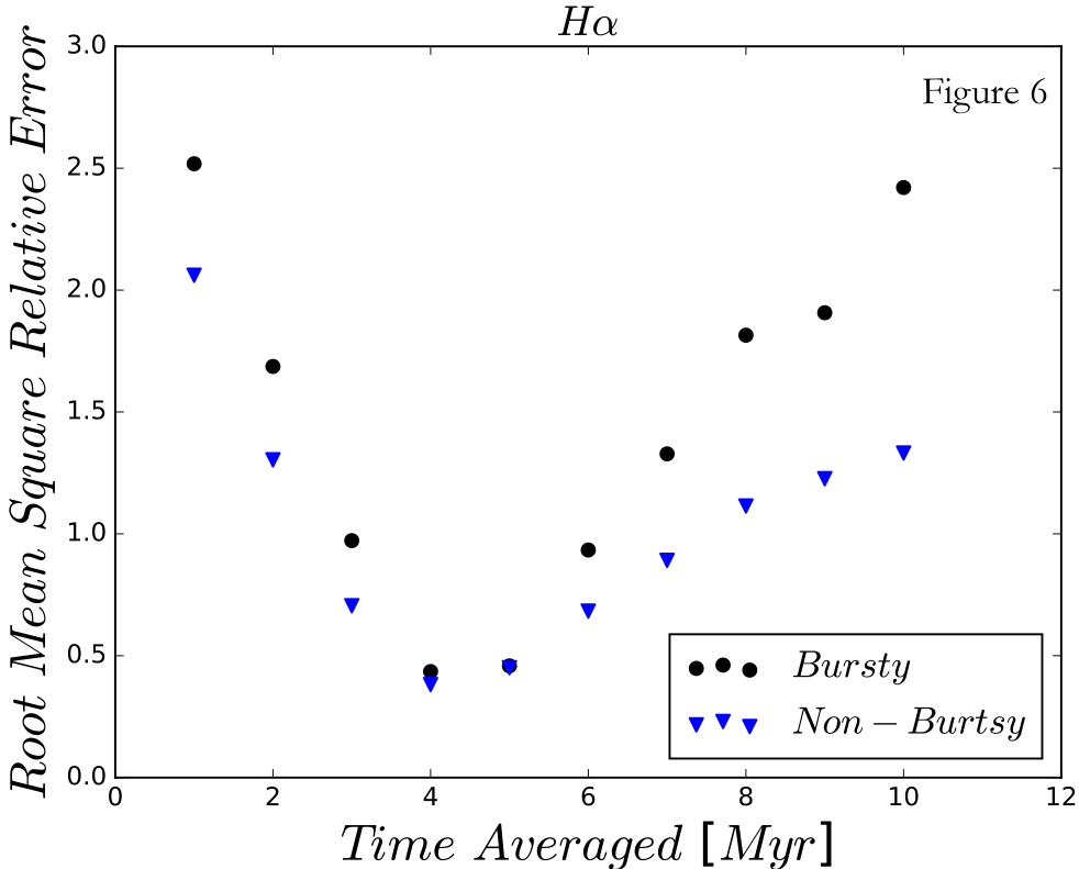
In this work we analyze observationally motivated indicators and compare to the true SFR of our simulated galaxy in these bursty and non-bursty epochs of SFR. In Figure 6 we find that the true SFR of our simulation best captures the Hα indicator when averaged over 4Myr. This plot was generated by recording the scatter quantity at averaged times scales from 1-10Myrs.

Future Work

Determine the averaged time scale which the true SFR best matches the SFR of the FUV indicator.

Expand our studies to different mass galaxies.

For further work on the project please visit my GitHub website as it will be updated as the research further progresses.