Our Model, the Simulation, and the Two Particle System

While we want our model to be as physically accurate as possible, we make some assumptions in order to lessen computational time and simplify the complex problem. First, we take orbits to be circular for ease of calculations. We believe that this is a reasonable assumption to be made for the sake of simplifying the calculations for the points of collision for the particles. We also acknowledge that orbital systems are very unpredictable, and we are not considering the gravitational attraction between the orbital particles. We also assume that momentum and mass are conserved.

In order to simulate these collisions, we need to determine when collisions are possible. The particles must be sufficiently close in radius, but determining what sufficiently close is in a simulation is difficult. We know that if a particle is in orbit, it must have negative energy; if the particle gains enough kinetic energy, it will overcome the gravitational attraction and leave orbit, effectively leaving our system. we can determine a constraint equation for the two radii based on this constraint in energy.

The final kinetic energy will be the average of the two initial kinetic energies, assuming the particles have equal energies after the collision. Assuming that the only energy present are gravitational and kinetic, in order to find the threshold value between negative and positive energy.

Additionally, the particles must be at the same angle about the orbit as one another. We can find the time of the next intersection between particles i and j as long as their radii are sufficiently close. We then find the smallest time interval within all the possible collisions, simulating the "first" collision.

Next, we consider the collision between particles i and j. For numerical simplification to our model, we assume that the masses of the particles are equal. We also take a reference frame that aligns particle $i$ with a horizontally directional initial velocity and particle j at a directional initial velocity an angle above the horizontal. When a collision occurs, by Newton's law of inertia, the system's momenta must be conserved. Using the assumptions above, we can draw conclusions about the momenta in the x and y directions of the two particles.

The Kuramoto model only applies to nonconservative systems, but we can assume that energy conservation is not obeyed. The collisions allow for the loss of energy through various possible avenues: heat loss into the surrounding environment, deformation of the particles, spin velocity that is not considered, etc. We assume that energy is being lost by a factor much less than one. We only consider the loss in kinetic energy here because the gravitational energies are similar. Our goal is to find the two final velocities components of both particles i and j; therefore, we must add another equation to our system: an equation describing the fractionation of the total final energy of particle i to the total final energy. We find the resultant velocities of particles i and j by solving the system of equations of x momentum, y momentum, energy loss, and energy fractionation. These final velocities are used to find the particles' resultant orbit levels, the frequencies after the collision, and the positions about the orbit using Kepler's planetary motion laws, correcting for the elliptical orbits assumed by assuming that there is only loss in the kinetic energy.

We continue to use this least-time-step method for a set amount of time, indicating that the system has had ample time to synchronize.

We can then measure the synchrony of the system of particles using Kuramoto's order parameter. Because we find the order parameter after every collision taking place, we want to average the order parameter over time so that we get a more holistic analysis of the system over time. This is an appropriate action because we expect an average over time to be more representative of a physical situation.

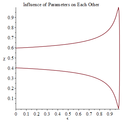
After creating the simulation, we studied the relationships between the parameters to ensure allowable ranges. First, we looked at the influence of the amount of lost energy on the distribution of energy between the two particles. We studied the simple case where the masses are equal and the initial velocities are equal in magnitude. When there is more energy lost, it is more reasonable to assume that the energy is distributed unevenly between the two particles colliding.