An Overview of the Simulation Process
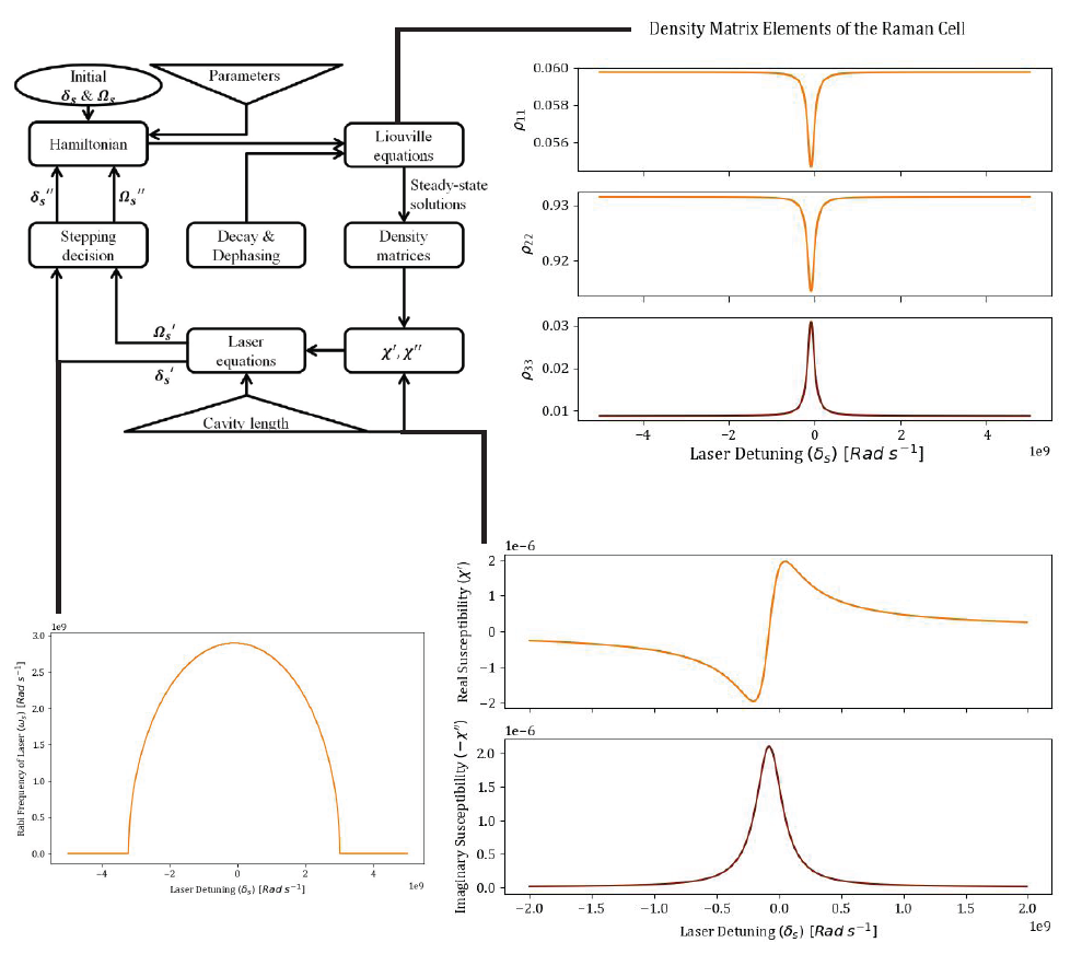
The first step in producing a subluminal laser model was to accurately find the steady state solution of the density matrix of any given intra-cavity medium since the diagonal elements of a density matrix for an atomic/molecular system provide the density of electrons in each of the energy levels. The evolution of the density matrix is governed by the Liouville equation and the steady state solution was found by implementing the general algorithm detailed in Shahriar et al. (2014) in Python. For the preliminary simulation of the subluminal laser , we only considered a laser containing a 0.1 m long Raman cell of Rubidium, which can be modeled as a three level system. The steady state solution was then used to calculate the real \(\chi'\) and imaginary \(\chi''\) of the effective susceptibility of the laser cavity. It is important to note that we considered the susceptibilities as functions of the signal (output) field's Rabi frequency \(\Omega_s\) and detuning \(\delta_s\) with respect to the |1> to |3> transition of Rubidium. These real and imaginary parts were then used to solve for the steady state of the single mode laser equation which give us the frequency and intensity of the subluminal laser (Zhou et al. 2016) , \begin{equation} \nu + \dot{\phi} = \Omega_c - \frac{\chi'}{2}\nu \end{equation} \begin{equation} \dot{E} = - \frac{\nu E}{2Q} - \frac{\chi'' E}{2}\nu \end{equation} where \(\nu\) is the lasing frequency, \(\phi\) is the phase of the lasing field, \(E\) is the amplitude of the lasing field, \(\Omega_c\) is the empty cavity resonant frequency, and Q is the quality factor of the cavity. In order to find a solution that simultaneously satisfied the Liouville equation, and both single-mode laser equations, we wrote an algorithm that iterates over \(\Omega_s\) and \(\delta_s\) pairs until it converges to a solution within the given tolerance. The frequency of the laser was then calculated using the equation (Zhou et al. 2016), \begin{equation} \nu = \nu_0 + \delta_{rp} + \delta_{s} \end{equation} where \(\nu_0\) is the nominal frequency of the transition used for lasing (795 nm in our case) and \(\delta_{rp}\) is the detuning of the Raman pump with respect to the |2> to |3> transition of Rubidium. The SSF of the laser was then calculated by running the complete algorithm for two different cavity lengths, calculating the difference in lasing frequency, and comparing to the difference in lasing frequency for an empty cavity given the same length change. A diagram of the modeling process and various outputs of the program are featured in Figure 4.